Extracting Pre-Post Correlations for Meta-Analyses of Repeated Measures Designs

In [1]:

library(tidyverse)

── Attaching core tidyverse packages ──────────────────────── tidyverse 2.0.0 ──
✔ dplyr     1.1.4     ✔ readr     2.1.5
✔ forcats   1.0.0     ✔ stringr   1.5.1
✔ ggplot2   3.5.1     ✔ tibble    3.2.1
✔ lubridate 1.9.3     ✔ tidyr     1.3.1
✔ purrr     1.0.2     
── Conflicts ────────────────────────────────────────── tidyverse_conflicts() ──
✖ dplyr::filter() masks stats::filter()
✖ dplyr::lag()    masks stats::lag()
ℹ Use the conflicted package (<http://conflicted.r-lib.org/>) to force all conflicts to become errors

library(ggdist)
library(MASS)

Attaching package: 'MASS'

The following object is masked from 'package:dplyr':

    select

library(cowplot)

Attaching package: 'cowplot'

The following object is masked from 'package:lubridate':

    stamp

library(latex2exp)

Introduction

Meta-analyses synthesizing studies using repeated measures designs are popular for drawing inferences about within-person effects over time or across conditions. While these meta-analyses are capable of providing insight into within-participant effects, when conducted improperly they can lead to biased results (Cuijpers et al. 2017). Specifically, repeated measures standardized mean differences (rmSMDs) tend to rely on pre-post correlations in their calculation (Table 1). However, these pre-post correlations are usually unavailable, leading meta-analysts to make inaccurate calculations. Some authors have gone so far as to recommend against the use of rmSMDs altogether (Cuijpers et al. 2017, 364):

We conclude that pre-post SMDs should be avoided in meta-analyses as using them probably results in biased outcomes.

Despite this cautionary stance, we advocate for a more nuanced approach. Numerous statistical methods are available to calculate pre-post correlations directly from alternative statistics, mitigating the risk of bias. Therefore, we believe that dismissing rmSMDs entirely may be an overly hasty response. Instead, we believe that this dilemma stems largely from the lack of clarity on when and how to use alternative statistics when calculating pre/post correlations for rmSMDs. Here we aim to establish a concise guide for calculating pre/post correlations depending on the available statistics (see Figure 1).

In [2]:

graph TB
    A((Pre-Post\n Correlation))
    S0(Scenario 0:\n Is the pre/post correlation or raw data available?) --No--> S1(Scenario 1:\n Is the change score standard\n deviation available?)
    S1 --No--> S2(Scenario 2:\n Is the SMD of change scores available?)
    S2 --No--> S3(Scenario 3:\n Is the paired t-statistic available?)
    S3 --No--> S4(Scenario 4:\n Is the p-value from a\n paired t-test available?)
    S4 --No--> S5(Scenario 5:\n Is a figure available?)
    S5 --No--> S6(Scenario 6:\n Is the standard deviation\n response ratios available?)
    S6 --No--> S7(Scenario 7:\n Is a Spearman or Kendall correlation\n coefficient available?)
    S7 --No--> S8(Scenario 8:\n Are there other similar studies\n with pre/post correlations?)
    S8 --No--> S9(Scenario 9:\n No usable information\n available)
    S9 --Rule of Thumb--> A
    S8 --Approximation--> A
    S7 --Approximation--> A
    S6 --Approximation--> A
    S5 --Almost\n Exact--> A
    S4 --Exact--> A
    S3 --Exact--> A
    S2 --Exact--> A
    S1 --Exact--> A
    S0 --Yes--> A

Figure 1: Decision tree-like diagram of pre-post calculation procedure. Denoted at the bottom with a circular node is the quantity of interest (i.e., the pre/post correlation). To follow the diagram, start at the upper-most node. Each node asks whether a specific type of information is available. If the information is not available, then move on to the next scenario, if the information is available, you will be able to estimate the pre/post correlation.

Defining the pre-post correlation

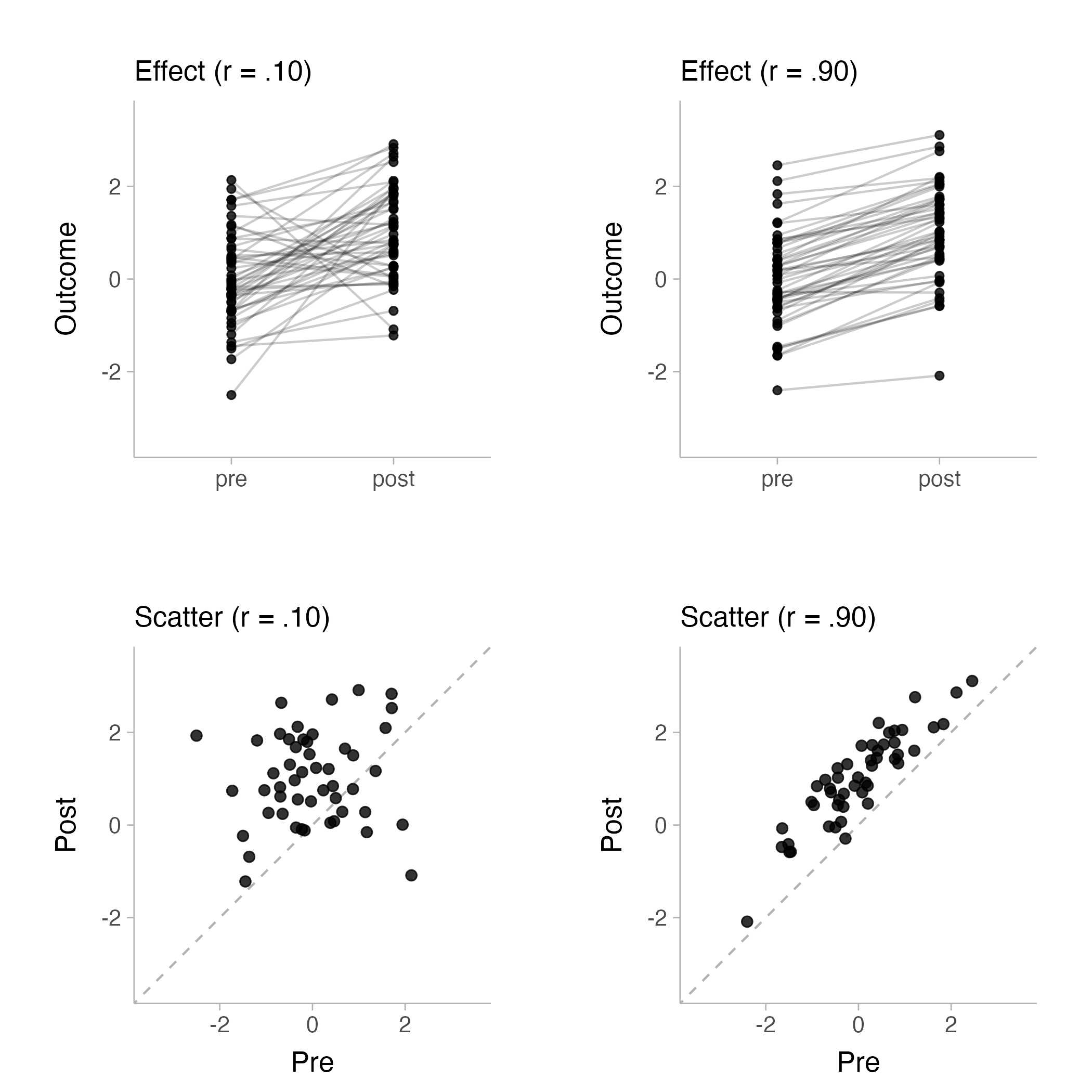
As we will see in the next section, pre-post correlations are present in the equations for rmSMDs. The pre-post correlation measures the stability of individual differences from pre to post intervention (see Figure 2). The population pre-post correlation is defined as the covariance (\(\sigma_{01} := \mathrm{cov}(Y_0,Y_1)\)) between pre \((Y_0)\) and post \((Y_1)\) intervention scores divided by the product of the standard deviations of pre \((\sigma_{0} := \sqrt{\mathrm{var}(Y_0)})\) and post \((\sigma_{1} := \sqrt{\mathrm{var}(Y_1)})\) intervention scores scores such that,

\[ \rho = \frac{\sigma_{01}}{\sigma_{0}\sigma_{1}}. \tag{1}\]

Within a sample, we can compute the Pearson’s product-moment estimator (Pearson and Filon 1897), which replaces the population values with the sample covariance \((s_{01})\) and standard deviations \((s_0\) and \(s_{1})\),

\[ r = \frac{s_{01}}{s_0 s_1} \tag{2}\]

Figure 2: Visualizing pre-post correlations with simulated data. Top row shows the pre-post change in scores for low (left) and high (right) correlations. Bottom row shows corresponding scatter plots for low (left) and high (right) pre-post correlations

Worked Example in R

Throughout the paper, we will use example data from the psychTools package (William Revelle 2024). This data set contains affect related scores of four groups at two time points. The four groups watched different films and then self-reported there affective states before and after their respective films. For this example, we will look at the difference in tense arousal scores before and after watching a horror movie. We can first load in the psychTools and tidyverse package (William Revelle 2024; Wickham et al. 2019).

In [3]:

library(psychTools)

Attaching package: 'psychTools'

The following object is masked from 'package:dplyr':

    recode

library(tidyverse)

After loading in the packages, we can then import the dataset, select for the necessary variables (i.e., tense arousal scores at pre TA1 and post TA2 as well as the film type Film), and filter out the films that are not of interest (i.e., all non-horror films). This results in a dataset of just the pre and post tense arousal scores for the horror movie condition only (first ten subjects of the dataset are displayed below).

In [4]:

# Load in data set
dat <- psychTools::affect %>%
  # Use scores at tense arousal scores only
  dplyr::select(Film, TA1, TA2) %>%
  # Rename TA1 to pretest and TA2 to posttest
  rename(pre = TA1, post = TA2) %>%
  # Only use film 2 (horror film)
  filter(Film == 2) %>%
  # Keep only pretest and posttest columns
  dplyr::select(pre,post)
  
# view first 10 subjects
head(dat,10)

   pre post
1   11   15
2    5    6
3    8   19
4    8   17
5   12   22
6   10   25
7   15   19
8   13   15
9    7   17
10  12   20

The correlation between pre-test and post-test scores is then simply calculated using the cor function in base R.

In [5]:

cor(dat$pre,dat$post)

[1] 0.4627346

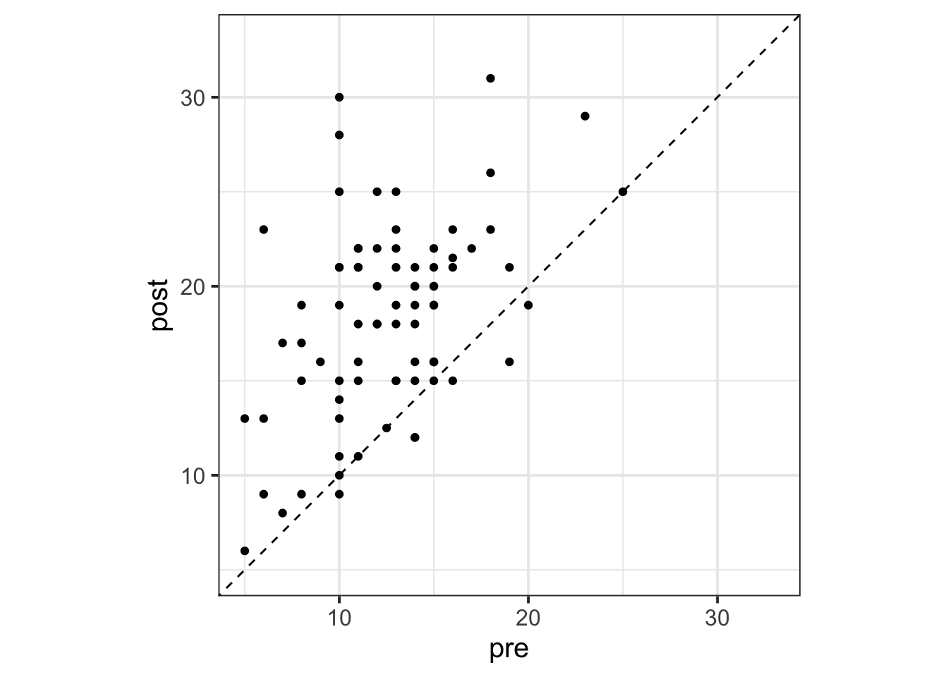
Therefore the correlation we will be estimating throughout the applied examples in this paper is \(r=0.46\). The pre-post correlation can be visualized by plotting out the pre intervention scores on the horizontal axis and the post intervention scores on the vertical axis.

In [6]:

# initialize ggplot object
ggplot(data = dat, aes(x = pre, y = post)) +
  # plot data points
  geom_point() +
  # set theme
  theme_bw(base_size=15) +
  # make axes square
  theme(aspect.ratio = 1) +
  # reference line
  geom_abline(intercept = 0, slope = 1, linetype = "dashed") +
  # set x and y limits
  lims(x=c(5,33), y=c(5,33))

Figure 3: Scatter plot displaying pre-post correlation. Reference line (dashed diagonal line) denotes equality between pre and post scores

Repeated Measures Standardized Mean Differences

Repeated Measures Standardized Mean Differences (rmSMDs) quantify the change in an outcome from pre to post intervention. There are various formulations of rmSMD (see Table 1) however they follow a similar algebraic expression. That is, the difference in the population post intervention mean (\(\mu_1\)) and the population pre intervention mean (\(\mu_0\)) divided by some standardizer (\(\sigma_*\)),

\[ \delta_* = \frac{\mu_1 - \mu_0}{\sigma_*}. \]

A sample estimator can be expressed similarly,

\[ d_* = \frac{m_1 - m_0}{s_*}, \]

where \(m_0\) and \(m_1\) are the sample means for the pre and post intervention scores, respectively. The standardizer (\(s_*\)) will be some type of standard deviation (e.g., standard deviation of change scores; see Table 1).

Table 1: Equations for the standardizer and sampling variance for different types of rmSMDs obtained from Jané et al. (2024). Note \(s_0\) = pre intervention standard deviation, \(s_1\) = post intervention standard deviation, \(r\) = pre-post correlation, \(n\) = sample size.

Estimator	Standardizer (\(s_*\))	Variance
Change score \(d_z\)	\[\sqrt{s^2_0+s^2_1-2rs_0s_1}\]	\[ \frac{1}{n} + \frac{d^2_z}{2n}\]
Repeated Measures \(d_{rm}\)	\[\sqrt{\frac{s^2_0 + s^2_1 - 2rs_0s_1}{2(1-r)}}\]	\[ \left(\frac{1}{n} + \frac{d^2_{rm}}{2n}\right) \times 2(1-r)\]
Average Variance \(d_{av}\)	\[\sqrt{\frac{s_0^2 + s_1^2}{2}}\]	\[\frac{2(s^2_0 + s^2_1 + 2rs_0s_1)}{n(s^2_0 + s^2_1)}\]
Baseline score \(d_b\)	\[s_0\]	\[\frac{2(1-r)}{n}+\frac{d^2_b}{2n}\]

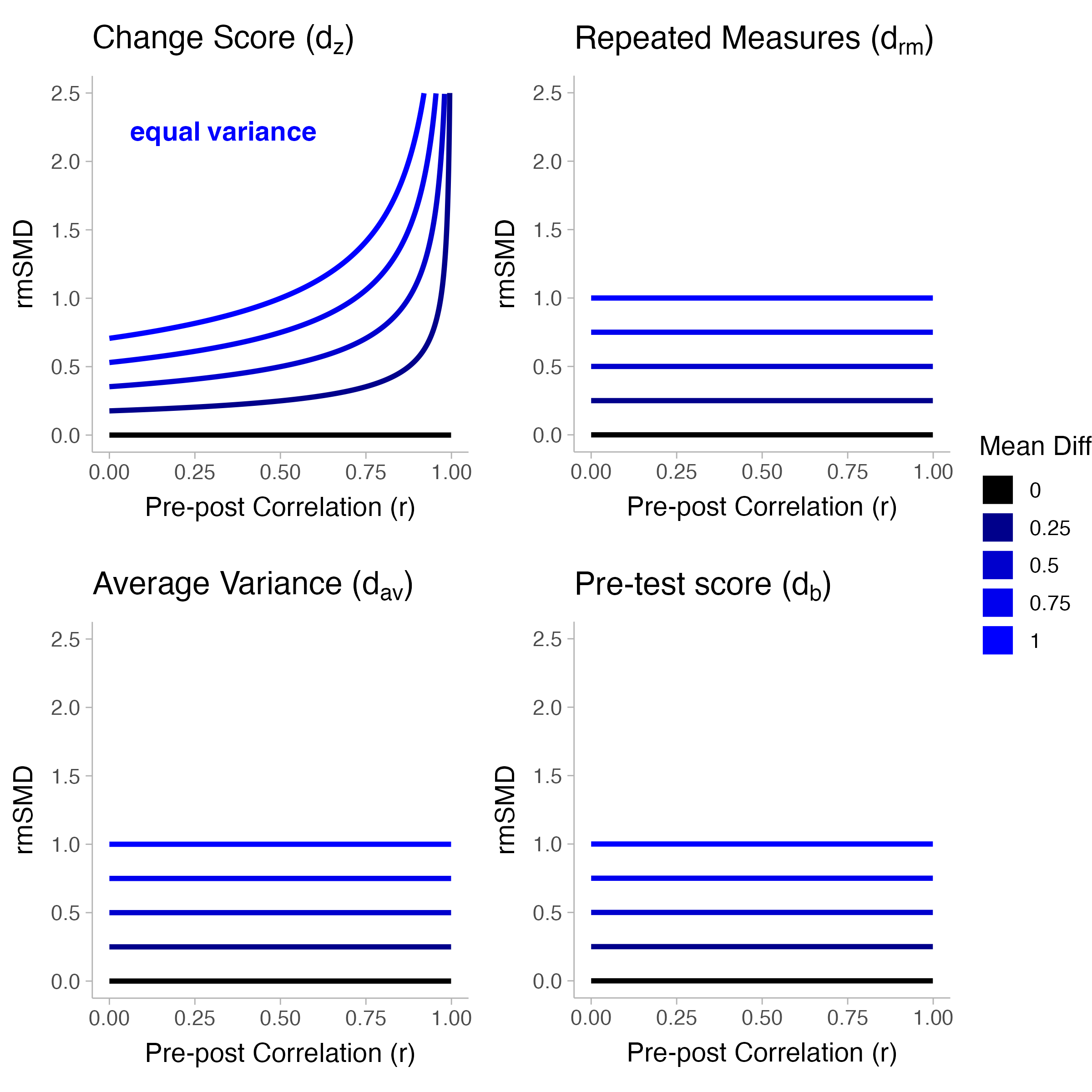
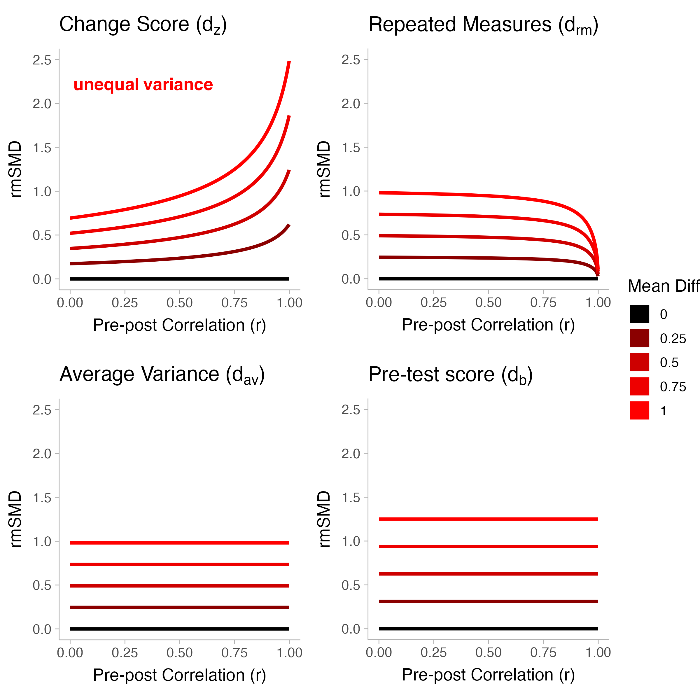
To decide on one of the four types of rmSMDs described in Table 1, one may want to consider a standardizer that does not contain the pre-post correlation (i.e., average variance \(d_{av}\) or baseline score \(d_b\)). This is due to the fact that changing the pre-post correlation can result in substantial changes to the rmSMD value even if there is no change in the raw mean difference (see Figure 4). For instance, the change score variant of the rmSMD (\(d_{z}\)) is highly influenced by the pre-post correlation even when the mean difference and variances are fixed (see first panel of Figure 4). On the other hand, like the change score variant of the rmSMD, the repeated measures variant (\(d_{rm}\)) contains the pre-post correlation in the standardizer (see Table 1). However, the pre-post correlation only has substantial influence on the value of \(d_{rm}\) if the variances are unequal between pre and post intervention (see Figure 5).

Figure 4: Repeated measures SMDs as a function of the pre-post correlation while varying the raw mean differences and fixing the standard deviations. The equal variance condition fixes the standard deviations in pre and post intervention to be one (\(\sigma_0=\sigma_1=1\)).

Figure 5: Repeated measures SMDs as a function of the pre-post correlation while varying the raw mean differences and fixing the standard deviations. The unequal variance condition sets different values for the standard deviations in pre (\(\sigma_0=0.8\)) and post intervention (\(\sigma_1=1.2\)).

Even if the pre-post correlation is not contained in the standardizer, it will be utilized in the sampling variance formula (see Table 1). Therefore, proper calculation of the rmSMD and it’s variance always requires the pre-post correlation.

Obtaining Pre/Post Correlations

Depending on what information is available to the meta-analyst the procedure for obtaining pre-post correlations varies. Here, we present a systematic procedure for calculating pre-post correlations. This procedure accounts for the differences in available information that a meta-analyst may come across in their literature review. Using a decision tree-like procedure (see Figure 1), we can prioritize exact methods of obtaining pre-post correlations rather than approximations, which become a last resort if all other information is unavailable. Each step in the diagram in Figure 1 will have a dedicated section in this paper overviewing the method given the available information.

Pre-post correlation calculation scenarios

Obtaining pre and post intervention means and standard deviations

For many of the following scenarios, calculations of the pre and post intervention mean and standard deviation will be required. While this is not always directly reported in primary studies, several common situations occur in which the mean and standard deviation can be obtained: 1) standard errors of the mean are reported instead of standard deviations, 2) confidence intervals of the mean are reported instead of standard deviations, 3) boxplots or five-point summaries are reported instead of means and standard deviations, 4) inter-quartile range and medians are reported instead of means and standard deviations 5) the min-max range is reported instead of standard deviations.

Standard errors to standard deviations

Standard deviations are calculable from the standard error of the mean (\(\mathrm{se}(m)\)) by multiplying the standard error by the square root of the sample size (\(n\)),

\[ s = \mathrm{se}(m)\times\sqrt{n}, \tag{3}\]

where \(se(m)\) is the standard error of the mean. It is pertinent to note that some primary studies may misreport standard deviations as standard errors and vice versa, so it is important to cross-check with other statistics (e.g., t-statistics).

Confidence intervals to standard deviations

The confidence interval (CI) of the sample mean can be converted to a standard deviation by taking the range of the confidence interval (\(CI_U-CI_L\), where the subscripts \(U\) and \(L\) denote the upper and lower bound) and first converting to a standard error. This is done by dividing the difference by the upper and lower CI by a factor containing the quantile function of the normal distribution and the false alarm rate (\(\alpha\)). This results in a standard error which can be multiplied by the square root of the sample size to obtain the standard deviation,

\[ s = \underset{\mathrm{se}(m)}{\underbrace{\frac{CI_{U} - CI_{L}}{2 \Phi^{-1}\!\left(1-\frac{\alpha}{2}\right)}}} \times \sqrt{n}. \tag{4}\]

Where \(\Phi^{-1}(\cdot)\) is the inverse of the cumulative distribution function of the standard normal distribution (in R, the qnorm() function is equivalent).

Boxplots and five-number summaries to means and standard deviations

If studies report distributions as a five-number summary (often displayed as a boxplot) with a minimum (\(\min(Y)\)), 25th percentile (\(q_1\)), median (\(q_2\); i.e., 50th percentile), 75th percentile (\(q_3\)), and maximum (\(\max(Y)\)) we can use these values to approximate the mean and standard deviation assuming an underlying normal distribution. To approximate the mean, we can use the following formula (Luo et al. 2018, eq. 15),

\[\begin{equation} \begin{aligned} m \approx &\left(\frac{2.2}{2.2+n^{.75}}\right) \frac{\min(Y) + \max(Y) }{2}\\ &+ \left(.7-\frac{.72}{n^{.55}}\right) \frac{q_1 + q_3}{2}\\ &+ \left(.3+\frac{.72}{n^{.55}}-\frac{2.2}{2.2+n^{.75}}\right) q_2. \end{aligned} \end{equation}\]

To approximate the standard deviation we can use the following formula (Shi et al. 2020, eq. 15),

\[\begin{equation} \begin{aligned} s \approx &\left(\frac{1}{1+.07 n^{.6}}\right)\frac{\max(Y) - \min(Y)}{2\Phi^{-1}\left(\frac{n-.375}{n+.25}\right)} \\ &+ \left(\frac{.07n^{.6}}{1+.07 n^{.6}}\right) \frac{q_3 - q_1}{2\Phi^{-1}\left(\frac{.75n-.125}{n+.25}\right)}. \end{aligned} \end{equation}\]

Although these formulas are quite complex, the conv.fivenum() function in the metafor R package (Viechtbauer 2010) can conduct these calculations easily.

Inter-quartile interval and median to means and standard deviations

If the author only reports the inter-quartile range (i.e., \([q_1,q_3]\)) rather than the five number summary, we use a different mean and standard deviation approximation using the following formulas (Wan et al. 2014, eq. 11 and 16, respectively).,

\[ m \approx \left(.7 + \frac{.39}{n}\right) \frac{q_3 + q_1}{2} + \left(.3 - \frac{.39}{n}\right)q_2 \]

\[ s \approx \frac{q_3 - q_2}{2\Phi^{-1}\left[\frac{.75n-.125}{n+.25}\right]} \]

The R function as mentioned before,conv.fivenum(), can calculate the mean and standard deviation from the sample size and the 25th, 50th (median), and 75th percentiles.

Min-max interval to means and standard deviations

If the full five-number summary is not reported and instead the primary study only reports the min-max interval (i.e., \([\min(Y),\max(Y)]\)) then we can calculate a different approximation for the mean and standard deviation (Luo et al. 2018, eq. 7; Wan et al. 2014, eq. 7)

\[ m \approx \left(\frac{4}{4+n^{.75}}\right) \frac{\max(Y) + \min(Y)}{2} + \left(\frac{n^{.75}}{4+n^{.75}}\right)q_2 \]

\[ s \approx \frac{\max(Y) - \min(Y)}{2\Phi^{-1}\left[\frac{n-.375}{n+.25}\right]} \]

The conv.fivenum() R function also has the ability to calculate the mean and standard deviation only from the sample size, minimum, maximum, and median.

Scenario 0: The pre/post correlation or raw data is reported.

This is the ideal scenario where the pre/post Pearson correlation is reported in the primary study or the raw data is available. If the correlation is not reported, but the raw data is available then we will have to calculate the pre/post correlation ourselves. This can be done easily in base R using the cor() function. If neither the raw data or Pearson correlation is available, contact the authors of the primary study to obtain the raw data.

Scenario 1: Is the change score standard deviation available?

Change scores (also known as gain scores or difference scores) are used to quantify the within subject change from pre to post intervention. They are simply the difference between a subject’s post intervention score and pre intervention score (\(Y_c = Y_1 - Y_0\)). If the study reports the standard deviation of change scores, then we can calculate the pre/post correlation with the following formula,

\[ r = \frac{s^2_0 + s^2_1 - s^2_c}{2s_0 s_1} \tag{5}\] Where \(s_c\) is the standard deviation of change scores. The derivation for Equation 5 can be found for Section 4. If the change score standard deviation is not reported, move on to Scenario 2.

Worked example in R

Let’s say a study reports the following summary statistic table containing the means and standard deviations for pre-test, post-test, and change scores for the tense arousal scale before and after watching a horror film (Table 2).

In [7]:

In [8]:

library(tinytable)

study_table <- data.frame(
  `Time` = c("Pre",
             "Post",
             "Change"),
  `Mean` = c(mean(dat$pre),
             mean(dat$post),
             mean(dat$pre-dat$post)),
  `SD` = c(sd(dat$pre),
           sd(dat$post),
           sd(dat$pre-dat$post)))

tt(study_table,digits=3)

Table 2: Reported statistics for tense arousal scores

Time	Mean	SD
Pre	12.62	3.84
Post	18.33	5.15
Change	-5.71	4.8

We can then use the formula in Equation 5 to compute the correlation exactly (within rounding error),

In [9]:

sd_pre <- 3.84
sd_post <- 5.15
sd_change <- 4.8

r <- (sd_pre^2 + sd_post^2 - sd_change^2) / (2*sd_pre*sd_post)

r

[1] 0.4608642

The correlation (almost) exactly matches the true value, however it is worth noting that the reported statistics will round to some decimal place so we will observe a some slight difference between the calculated pre-post correlation value (\(r = 0.461\)) and the actual value (\(r = 0.463\)).

Scenario 2: Is the change score rmSMD available?

The change score rmSMD (\(d_z\)) is the mean change (\(m_c = m_2 - m_1\)) between pre and post intervention scores divided by the change score standard deviation (\(s_c\); see the first estimator in Table 1). Using the change score rmSMD we can compute the pre-post correlation with the following formula,

\[ r = \frac{s^2_0 + s^2_1 - \left(\frac{m_c}{d_z}\right)^2}{2s_0 s_1}. \tag{6}\]

For the derivation of this equation see Section 5. If the change score rmSMD is not available, move on to scenario 3.

Worked example in R

Let’s say a study reports the following table in the results section containing the means and standard deviations for pre-test, post-test, and rmSMD (\(d_z\)) for the tense arousal scale before and after watching a horror film (Table 2).

In [10]:

In [11]:

library(tinytable)

study_table <- data.frame(
  Pre.Mean = mean(dat$pre),
  Pre.SD = sd(dat$pre),
  Post.Mean = mean(dat$post),
  Post.SD = sd(dat$post),
  dz = c(mean(dat$post-dat$pre) /
             sd(dat$post-dat$pre))
)

tt(study_table,digits=4)

Table 3: Reported results for horror film effect on tense arousal scores

Pre.Mean	Pre.SD	Post.Mean	Post.SD	dz
12.62	3.845	18.33	5.155	1.191

In R, we can use the values from this table to compute the pre-post correlation from the formula described in Equation 6,

In [12]:

mean_pre <- 12.62
sd_pre <- 3.845
mean_post <- 18.33
sd_post <- 5.155
dz <- 1.191

r <- (sd_pre^2 + sd_post^2 - ((mean_post - mean_pre)/dz)^2) /
  (2 * sd_pre * sd_post)

r

[1] 0.4634693

The calculated correlation (\(r = 0.463\)) precisely reflects the actual correlation (\(r =0.463\)).

Scenario 3: Is the t-statistic from a paired t-test available?

The paired t-statistic (\(t\)) is the test statistic for the paired t-test. It is calculated by the ratio of the mean change (\(m_c = m_2 - m_1\)) divided by the standard error of the mean of change scores (\(t=m_c/\mathrm{se}(m_c)\)). If the study reports the t-statistic then we can calculate the pre-post correlation with the following formula,

\[ r = \frac{t^2(s^2_0 + s^2_1)-n\times m^2_c}{2t^2s_0s_1} \tag{7}\]

Note that the paired t-statistic is equal to the square root of an F-statistic from a one-way ANOVA with two groups (\(t=\sqrt{F}\)). For the derivation of Equation 7 see Section 6. If the t-statistic is not available, move on to scenario 4.

Worked example in R

Continuing with the example involving the effect of a horror film on tense arousal scores, let’s suppose a study reports the following table (Table 4). The table reports the t-statistic from a paired t-test along with the pre and post means and standard deviations of tense arousal scores.

In [13]:

In [14]:

study_table <- data.frame(
  Pre.Mean = mean(dat$pre),
  Pre.SD = sd(dat$pre),
  Post.Mean = mean(dat$post),
  Post.SD = sd(dat$post),
  t.val = t.test(x = dat$post, 
         y = dat$pre, 
         paired=TRUE)$statistic,
  N = nrow(dat)
)

tt(study_table,digits = 4)

Table 4: Paired t-test results

Pre.Mean	Pre.SD	Post.Mean	Post.SD	t.val	N
12.62	3.845	18.33	5.155	10.52	78

In R, we can use the formula from Equation 7 to compute the pre/post correlation.

In [15]:

pre_mean <- 12.62
pre_sd <- 3.845
post_mean <- 18.33
post_sd <- 5.155
paired_t <- 10.52
n <- 78


r <- (paired_t^2*(sd_pre^2 + sd_post^2)-n*(post_mean-pre_mean)^2) /
  (2*paired_t^2*sd_pre*sd_post)
r

[1] 0.4636207

The computed correlation (\(r = 0.464\)) is an precise calculation of the actual pre-post correlation (\(r =0.463\)).

Scenario 4: Is the p-value from a paired t-test reported?

Sometimes the paired t-statistic is not provided and instead the study reports the p-value (\(p\)) associated with the paired t-test. Using the inverse cumulative distribution function of the Student’s t distribution (\(\Phi^{-1}_t(q,\nu)\), where \(q\) indicates the quantile and \(\nu\) denotes the degrees of freedom) we can compute the t-statistic and thus the pre-post correlation,

\[ r = \frac{\Phi^{-1}_t (p/2,n-1)^2\times (s^2_1 + s^2_2)-n\times m^2_c}{2\Phi^{-1}_t (p/2,n-1)^2\times s_1s_2} \tag{8}\]

See the derivation of this formula in Section 7. Similarly, a pre-post correlation can also be obtained from a one-tailed t-test,

\[ r = \frac{\Phi^{-1}_t (p,n-1)^2\times (s^2_1 + s^2_2)-n\times m^2_c}{2\Phi^{-1}_t (p,n-1)^2\times s_1s_2} \]

If the p-value is not available, move on to scenario 5.

Worked example in R

Let’s the following table was reported in the results section of a study (see Table 5). This time, the study only reports the p-value from a two-tailed paired t-test.

In [16]:

In [17]:

study_table <- data.frame(
  Pre.Mean = mean(dat$pre),
  Pre.SD = sd(dat$pre),
  Post.Mean = mean(dat$post),
  Post.SD = sd(dat$post),
  p.val = round(t.test(x = dat$post, 
         y = dat$pre, 
         paired=TRUE)$p.value,17),
  N = nrow(dat)
)

tt(study_table,digits = 4)

Table 5: Study results of paired t-test between pre- and post-test mean tense arousal scores.

Pre.Mean	Pre.SD	Post.Mean	Post.SD	p.val	N
12.62	3.845	18.33	5.155	1.5e-16	78

Using Equation 8 we can compute the pre-post correlation.

In [18]:

pre_mean <- 12.62
pre_sd <- 3.845
post_mean <- 18.33
post_sd <- 5.155
pval <- 1.5e-16 # from a paired t-test
n <- 78

# get paired t from p value
paired_t <- qt(pval/2, n-1, lower.tail = FALSE)

r <- (paired_t^2*(sd_pre^2 + sd_post^2)-n*(post_mean-pre_mean)^2) /
  (2*paired_t^2*sd_pre*sd_post)

The computed correlation (\(r = 0.463\)) is an exact calculation of the actual pre-post correlation (\(r =0.463\)).

Scenario 5 (almost exact): Is a figure available with the necessary information?

Figures can convey a lot of information that goes unreported in the primary text. If a figure contains the information needed to calculate the pre-post correlation, then meta-analysts can use plot digitizers such as WebPlotDigitizer (Rohatgi 2022) to extract the necessary data. If a figure is not available, move on to scenario 6.

Scenario 6 (approximation): Is an alternative correlation coefficient available (i.e., Spearman’s or Kendall’s correlation)?

If the pre-post correlation is reported as a Spearman rank-order correlation, we can use the Spearman correlation (\(r_\mathrm{s}\)) to approximate the Pearson correlation assuming the data follows a bivariate normal distribution (Rupinski and Dunlap 1996, eq. 2), \[ r \approx 2\sin^{-1}\left(\frac{\pi \times r_\mathrm{s}}{6}\right). \tag{9}\] However, if the pre-post correlation is reported as a Kendall’s \(\tau\) coefficient (\(r_\tau\)), we can use Kendall’s (1962) formula for converting to a Pearson correlation (assuming an underlying bivariate normal distribution), \[ r \approx \sin^{-1}\left(\frac{\pi\times r_\tau}{2}\right). \tag{10}\] If both \(r_\mathrm{s}\) and \(r_\tau\) are available, use the Spearman approximation formula in Equation 9 as we show in Section 2.8.2 the Kendall approximation and the midpoint of the two have slightly more approximation error. If neither are available, move on to scenario 7.

Worked example in R

In [19]:

spearman_r <- cor(dat$pre,dat$post, 
                 method = "spearman")

spearman_r_intext <- paste0("$",round(spearman_r,2),"$")

Using the horror film example, let’s say a study reports the pre-post correlation as a Spearman rank-order correlation (\(r_\mathrm{s}=\) \(0.39\)). Assuming an underlying bivariate normal distribution, we can make a reasonable estimate of the Pearson pre-post correlation simply by using Equation 9.

In [20]:

# approximation from spearman's correlation
spearman_r <- .39
r_approx <- 2*asin(pi*spearman_r/6)

r_approx

[1] 0.4113

As we can see from the code output, the resulting approximate Pearson pre-post correlation turns out to be 0.41 which is very close to the actual value (0.46).

Simulation check: midpoint of Spearman and Kendall approximation

To assess whether taking the midpoint of the two approximations performs better than either approximation alone, we simulate bivariate normal data with a population correlation of .5 and see if the midpoint of the Spearman and Kendall approximations (i.e., \(r \approx \frac{1}{2}\left[2\sin^{-1}\left(\frac{\pi \times r_\mathrm{s}}{6}\right) + \sin^{-1}\left(\frac{\pi\times r_\tau}{2}\right)\right]\)) has lower error than both the Spearman (Equation 9) and Kendall (Equation 10) approximations alone. Over 10,000 iterations, the absolute error was lowest in the Spearman approximation when compared to both the Kendall approximation and the midpoint of both (see Table 6).

In [21]:

In [22]:

library(MASS)

true_r <- c()
kendall_r <- c()
spearman_r <- c()

for(i in 1:10000){
  data <- mvrnorm(n = 50,
                mu = c(0,0), 
                Sigma = data.frame(x = c(1,.5),y=c(.5,1)))
  
  true_r[i] <- cor(data[,1],data[,2])
  kendall_r[i] <- asin(pi*cor(data[,1],data[,2],method = "kendall")/2)
  spearman_r[i] <- 2*asin(pi*cor(data[,1],data[,2],method = "spearman")/6)
}

midpoint_r <- .5 * (kendall_r + spearman_r)

results<- data.frame(
  midpoint = mean(abs(midpoint_r - true_r)),
  spearman = mean(abs(spearman_r - true_r)),
  kendall = mean(abs(kendall_r - true_r))
)

tinytable::tt(results,digits = 4) |>
  group_tt(j = list("Mean Absolute Error" = 1:3))

Table 6: Simulation results

Mean Absolute Error
midpoint	spearman	kendall
0.05449	0.03859	0.07718

Scenario 7 (approximation): Is the standard deviation of response ratios available?

Sometimes primary studies report pre-post change as a ratio of post intervention scores to pre intervention scores (\(Y_\mathrm{ratio} = Y_2/Y_1\)). Since the variance of a ratio depends on the pre-post correlation, we can use the variance of the response ratio to obtain the pre-post correlation. There is no closed form solution to the standard deviation of a ratio (\(s_\mathrm{ratio}\)), therefore an approximation (via a Taylor series expansion) of the pre-post correlation is given below:

\[ r\approx -\frac{m_1m_2}{2s_1s_2}\left(s_\mathrm{ratio}^2 \frac{m^2_1}{m^2_2}- \frac{s^2_1}{m_1^2} - \frac{s^2_2}{m_2^2}\right). \tag{11}\]

See the derivation of this formula in Section 8. If the standard deviation of the ratio is not available then move on to Scenario 7.

Worked example in R

Continuing with the anxiety example, imagine we are given the table in Table 7.

In [23]:

In [24]:

df <- data.frame(Time = c("Pre-test","Post-test", "Ratio"),
                 Mean = c(mean(dat$pre), 
                          mean(dat$post), 
                          mean(dat$post/dat$pre)),
                 SD =   c(sd(dat$pre), 
                          sd(dat$post), 
                          sd(dat$post/dat$pre)))

tinytable::tt(df,digits = 2)

Table 7: Reported means, SDs, and response ratios for pre/post effect

Time	Mean	SD
Pre-test	12.6	3.84
Post-test	18.3	5.15
Ratio	1.5	0.54

Then we can use these values to calculate an approximation of the pre/post correlation.

In [25]:

mean_pre <- 12.6
sd_pre <- 3.84
mean_post <- 18.3
sd_post <- 5.15
mean_ratio <- 1.50
sd_ratio <- .54

r <- -(mean_pre*mean_post)/(2*sd_pre*sd_post) *
  ((sd_ratio^2*mean_pre^2)/(mean_post^2) -
     (sd_pre^2)/(mean_pre^2) -
     (sd_post^2)/(mean_post^2))
r

[1] 0.197279

Note that this method is a rough approximation and may differ substantially from the actual value of the pre/post correlation as we see here. The computed value (\(r = 0.197\)) differs substantially than the actual value (\(r =0.463\)).

Simulation check of approximation formula

The formula in Equation 11 comes from solving for the correlation from the Taylor series approximation of the variance of a ratio by Seltman (n.d.). This is a pdf found on a university website and is not peer-reviewed, therefore this section will check the accuracy of the approximation.

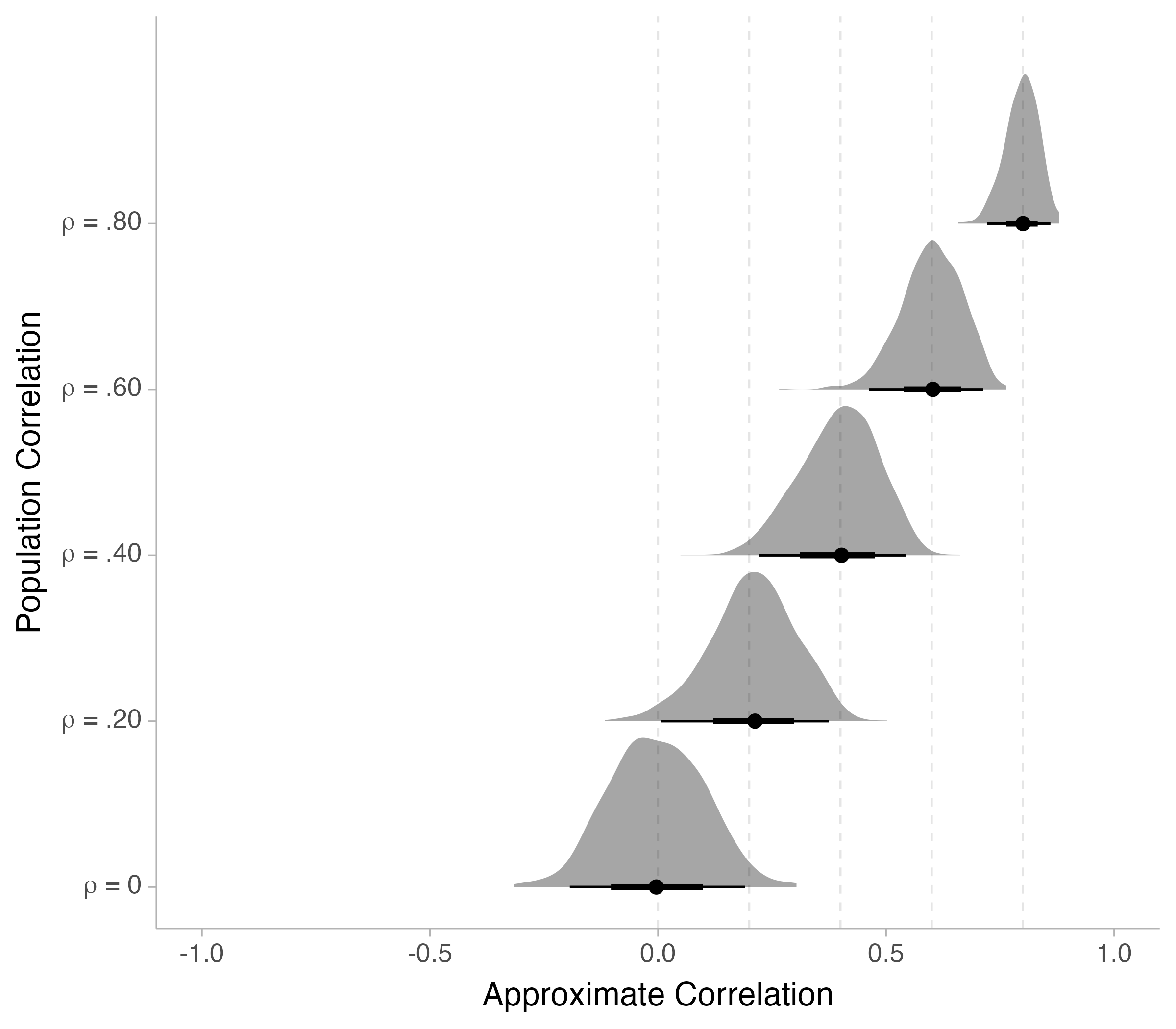
For this simulation we will generate data from a bivariate normal distribution (pre intervention mean = 100, post intervention mean = 101, pre intervention standard deviation = 1, post intervention standard deviation = 1) with a sample size of 100 and evaluated at correlation values of 0, .20, .40, .60, and .80. The approximation will be computed on 1,000 iterations at each correlation value.

The results (visualized in Figure 6) of the simulation show that the sampling distribution is properly calibrated to the population correlation for each and every condition. The sampling variances of the approximated correlations also were just slightly larger than what we would expect (see Table 8)

Figure 6: Sampling distributions of approximate pre/post correlations from Equation 11 5 conditions with varying population correlations.

In [26]:

In [27]:

source("Figure_sim.R")
app_means <- summarize(r_app,
                       mean_r_0 = mean(V1),
                       mean_r_2 = mean(V2),
                       mean_r_4 = mean(V3),
                       mean_r_6 = mean(V4),
                       mean_r_8 = mean(V5))

app_vars <- summarize(r_app,
                      var_r_0 = var(V1),
                      var_r_2 = var(V2),
                      var_r_4 = var(V3),
                      var_r_6 = var(V4),
                      var_r_8 = var(V5))
expected_means <- rho
  
expected_vars <- c(((1-rho[1]^2)^2)/100,
                  ((1-rho[2]^2)^2)/100,
                  ((1-rho[3]^2)^2)/100,
                  ((1-rho[4]^2)^2)/100,
                  ((1-rho[5]^2)^2)/100)

sim.table <- data.frame(t(app_means),expected_means,
                        t(app_vars),expected_vars) |>
  set_names(c("Approximation","Expected",
              "Approximation","Expected"))
options(tinytable_tt_digits = 3)
tt(sim.table,digits = 2) |> 
  group_tt(j = list("Means" = 1:2, "Variance" = 3:4))

Table 8: Simulation results

Means		Variance
Approximation	Expected	Approximation	Expected
-0.0026	0	0.0106	0.01
0.2082	0.2	0.0087	0.0092
0.3962	0.4	0.0072	0.0071
0.5995	0.6	0.0044	0.0041
0.7974	0.8	0.0013	0.0013

Scenario 8 (approximation): Are there other similar studies with pre-post correlations?

If there is no usable information to calculate the pre-post correlation within the study of interest, then we can use information from similar studies to make a reasonable approximation. If we have pre-post correlations from \(k\) studies, we can conduct a fixed effects meta-analysis to calculate the average pre-post correlation and then use it as an estimate for the current study. The correlation estimate can be obtained by following a three-step procedure: 1) transform the Pearson correlations to Fisher’s Z correlations (i.e., hyperbolic arctangent transform), 2) compute a inverse-variance weighted average of the available Fisher’s Z correlations, and 3) back-transform the average Fisher’s Z correlation to a Pearson correlation. We can combine these three steps into a single equation,

\[ r \approx \bar{r} = \tanh\left[\frac{\sum^k_{i=1} (n_i-3) \tanh^{-1} (r_{i}) }{\sum^k_{i=1} (n_i-3)}\right], \] where \(n_i\) and \(r_i\) are the sample size and correlation for study \(i\), respectively. If there are no studies that provide pre-post correlations, then move on to Scenario 8.

Example in R

To compute the average correlation in R, we will need the sample sizes and sample correlations from each study. For this example, we will suppose there are three studies with correlations of .42, .61, and .33 with sample sizes 41, 18, and 34, respectively.

In [28]:

sample_r <- c(.42,.61,.33) # sample correlations
n <- c(41, 18, 34) # sample sizes

# n-weighted averaged correlation
r <- tanh(sum((n-3)*atanh(sample_r)) / sum(n-3))

r

[1] 0.4265244

The mean correlation is estimated to be \(r = 0.427\) where the true correlation for that study is \(r =0.463\).

Scenario 9: No usable information available

In the worst case scenario where the current study and no other studies provide any information on the pre-post correlations, we recommend using multiple values of the pre-post correlation (e.g., \(r=.25,.50,.75\)) and conduct sensitivity analyses. At this stage, it is important to emphasize the use of rmSMDs that do not contain the pre-post correlation in their calculation (i.e., \(d_{av}\) and \(d_{b}\)). Although the sampling variance will still contain the pre-post correlation, we can at least mitigate potential bias in the rmSMD estimates.

Conclusion

Conducting meta-analyses on repeated measures designs poses a common hurdle: the scarce reporting of pre-post correlations. In response to this challenge, we have introduced a series of equations designed to facilitate the extraction of pre-post correlations from alternative statistical information. Each equation is created to align with distinct scenarios, accommodating varying combinations of available statistics that meta-analysts may encounter.

These scenarios are systematically arranged from the most favorable, denoted as Scenario 0, to the least favorable, represented by Scenario 9. This structure helps to prioritize easier and exact conversions over approximations. It also serves as a practical guide for meta-analysts seeking solutions when confronted with inconsistent statistical information.

Scenario 1: Derivation

Change scores denote the difference between a subject’s post and pre intervention scores (\(Y_c = Y_1 - Y_0\)). The variance of a change score (\(\sigma_c\)) is defined as,

\[ \sigma^2_c = \sigma^2_0 + \sigma^2_1 - 2\sigma_{01} \]

The covariance between pre and post intervention scores (\(\sigma_{01}\)) can be expressed in terms of the pre-post correlation. Therefore, we can replace \(\sigma_{01}\) with \(\rho_{01}\sigma_0\sigma_1\),

\[ \sigma^2_c = \sigma^2_0 + \sigma^2_1 - 2\rho\sigma_0\sigma_1. \]

Solving for the pre-post correlation (\(\rho\)) will give us the following equation,

\[ \rho = \frac{\sigma^2_0 + \sigma^2_1 - \sigma^2_c}{2\sigma_0\sigma_1}. \tag{12}\]

Thus the sample pre-post correlation is analogously defined as,

\[ r = \frac{s^2_0 + s^2_1 - s^2_c}{2s_0 s_1} \]

Scenario 2: Derivation

The change score rmSMD can be defined as the difference in means between pre and post intervention scores or, equivalently, the mean of change scores (\(\mu_c = \mu_1-\mu_0\)) divided by the change score standard deviation (\(\sigma_c\)),

\[ \delta_z = \frac{\mu_1 - \mu_0}{\sigma_c} = \frac{\mu_c}{\sigma_c} \]

Solving for the change score standard deviation gives,

\[ \sigma_c = \frac{\mu_1-\mu_0}{\delta_z} = \frac{\mu_c}{\delta_z}. \]

This can then be plugged into Equation 12,

\[ \rho = \frac{\sigma^2_0 + \sigma^2_1 - \sigma_c^2}{2\sigma_0\sigma_1} = \frac{\sigma^2_0 + \sigma^2_1 - \left(\frac{\mu_c}{\delta_z}\right)^2}{2\sigma_0\sigma_1}. \]

Therefore the sample pre-post correlation can be calculated as,

\[ r = \frac{s^2_0 + s^2_1 - \left(\frac{m_c}{d_z}\right)^2}{2s_0s_1}. \]

Scenario 3: Derivation

The paired t-statistic can be expressed in terms of the change score standard deviation such that,

\[ t = \frac{m_c}{\mathrm{se}(m_c)} = \frac{m_c}{\left(\frac{s_c}{\sqrt{n}}\right)}= \frac{m_c\times \sqrt{n}}{s_c} \]

Solving for the change score standard deviation gives,

\[ s_c = \frac{m_c\times \sqrt{n}}{t} \]

Plugging this into Equation 5 yields,

\[ r = \frac{s^2_0 + s^2_1 - s_c^2}{2s_0 s_1}= \frac{s^2_0 + s^2_1 - \left(\frac{m_c\times \sqrt{n}}{t}\right)^2}{2s_0 s_1} \] Simplifying this gives,

\[ r = \frac{t^2(s^2_0 + s^2_1)-n\times m^2_c}{2t^2s_0s_1} \tag{13}\]

Scenario 4: Derivation

The paired t-statistic for a two-tailed paired t-test can be calculated from a p-value by using the inverse cumulative Student’s t distribution (\(\Phi^{-1}_t [q,\nu]\), where \(q\) is the quantile and \(\nu\) is the degrees of freedom),

\[ t = \Phi^{-1}_t \left[p/2,n-1\right] \]

Plugging this into Equation 13 yields,

\[ r = \frac{t^2(s^2_0 + s^2_1)-n\times m_c}{2t^2s_0s_1} = \frac{\Phi^{-1}_t [p/2,n-1]^2\times (s^2_0 + s^2_1)-n\times m_c}{2\Phi^{-1}_t [p/2,n-1]^2\times s_0s_1} \]

Scenario 6: Derivation

An approximation of the variance of a ratio between two random variables was derived by Seltman (n.d.). For our case,

\[ \sigma_\mathrm{ratio}^2 \approx \frac{\mu^2_1}{\mu^2_0} \left(\frac{\sigma^2_0}{\mu_0^2} + \frac{\sigma^2_1}{\mu_1^2} - 2\frac{\rho\sigma_0\sigma_1}{\mu_0\mu_1}\right) \]

We can then solve for the pre/post correlation,

\[ \rho\approx -\frac{\mu_0\mu_1}{2\sigma_0\sigma_1}\left(\sigma_\mathrm{ratio}^2 \frac{\mu^2_0}{\mu^2_1}- \frac{\sigma^2_0}{\mu_0^2} - \frac{\sigma^2_1}{\mu_1^2}\right) \]

For a sample, this can be written as,

\[ r\approx -\frac{m_0m_1}{2s_0s_1}\left(s_\mathrm{ratio}^2 \frac{m^2_0}{m^2_1}- \frac{s^2_0}{m_0^2} - \frac{s^2_1}{m_1^2}\right) \]

Cuijpers, P., E. Weitz, I. A. Cristea, and J. Twisk. 2017. “Pre-Post Effect Sizes Should Be Avoided in Meta-Analyses.” Epidemiology and Psychiatric Sciences 26 (4): 364–68. https://doi.org/10.1017/S2045796016000809.

Jané, Matthew B., Qinyu Xiao, Siu Kit Yeung, Mattan Ben Shachar, Aaron Caldwell, Denis Cousineau, Daniel Dunleavy, et al. 2024. Guide to Effect Sizes and Confidence Intervals. https://doi.org/10.17605/OSF.IO/D8C4G.

Kendall, Maurice George. 1962. Rank Correlation Methods. Griffin.

Luo, Dehui, Xiang Wan, Jiming Liu, and Tiejun Tong. 2018. “Optimally Estimating the Sample Mean from the Sample Size, Median, Mid-Range, and/or Mid-Quartile Range.” Statistical Methods in Medical Research 27 (6): 1785–805. https://doi.org/10.1177/0962280216669183.

Pearson, Karl, and L. N. G. Filon. 1897. “Mathematical Contributions to the Theory of Evolution. IV. On the Probable Errors of Frequency Constants and on the Influence of Random Selection on Variation and Correlation. [Abstract].” Proceedings of the Royal Society of London 62: 173–76. https://www.jstor.org/stable/115709.

Rohatgi, Ankit. 2022. “Webplotdigitizer: Version 4.6.” https://automeris.io/WebPlotDigitizer.

Rupinski, Melvin T., and William P. Dunlap. 1996. “Approximating Pearson Product-Moment Correlations from Kendall’s Tau and Spearman’s Rho.” Educational and Psychological Measurement 56 (3): 419–29. https://doi.org/10.1177/0013164496056003004.

Seltman, Howard. n.d. “Approximations for Mean and Variance of a Ratio.” https://www.stat.cmu.edu/~hseltman/files/ratio.pdf.

Shi, Jiandong, Dehui Luo, Hong Weng, Xian-Tao Zeng, Lu Lin, Haitao Chu, and Tiejun Tong. 2020. “Optimally Estimating the Sample Standard Deviation from the Five-Number Summary.” Research Synthesis Methods 11 (5): 641–54. https://doi.org/10.1002/jrsm.1429.

Viechtbauer, Wolfgang. 2010. “Conducting Meta-Analyses in R with the metafor Package.” Journal of Statistical Software 36 (3): 1–48. https://doi.org/10.18637/jss.v036.i03.

Wan, Xiang, Wenqian Wang, Jiming Liu, and Tiejun Tong. 2014. “Estimating the Sample Mean and Standard Deviation from the Sample Size, Median, Range and/or Interquartile Range.” BMC Medical Research Methodology 14 (1): 135. https://doi.org/10.1186/1471-2288-14-135.

Wickham, Hadley, Mara Averick, Jennifer Bryan, Winston Chang, Lucy D’Agostino McGowan, Romain François, Garrett Grolemund, et al. 2019. “Welcome to the tidyverse.” Journal of Open Source Software 4 (43): 1686. https://doi.org/10.21105/joss.01686.

William Revelle. 2024. psychTools: Tools to Accompany the ’Psych’ Package for Psychological Research. Evanston, Illinois: Northwestern University. https://CRAN.R-project.org/package=psychTools.