library(metafor)
library(ggdist)
library(tidyverse)
library(clubSandwich)
library(MASS)
library(ggdist)
theme_set(theme_ggdist(base_size=15))Error Report #1
Study Title: Mindfulness-Based Stress Reduction for Stress Management in Healthy People: A Review and Meta-Analysis
Journal: The Journal of Alternative and Complementary Medicine
DOI: 10.1089/acm.2008.0495
Citations: 2879
Summary: The meta-analysis by Chiesa and Serretti (2009) contains substantial data extraction errors (i.e., effect size calculation errors) and analysis flaws that artificially inflate the difference between treatment and control pre-post effects. In this report I walk through each of the calculations for all studies included in the meta-analysis that I have access to. Due to the severe data extraction errors and analysis flaws, all the meta-analytic results in Chiesa and Serretti (2009) are incorrect and exaggerate the effect between MBSR and control groups for both stress and spirituality outcomes.
Load necessary R packages
Let’s first load in packages for the analysis.
Tabulating Table 1 of Chiesa and Serretti (2009)
First we will extract the information from table 1 from Chiesa and Serretti (2009). Here is the screenshot of table 1 below:
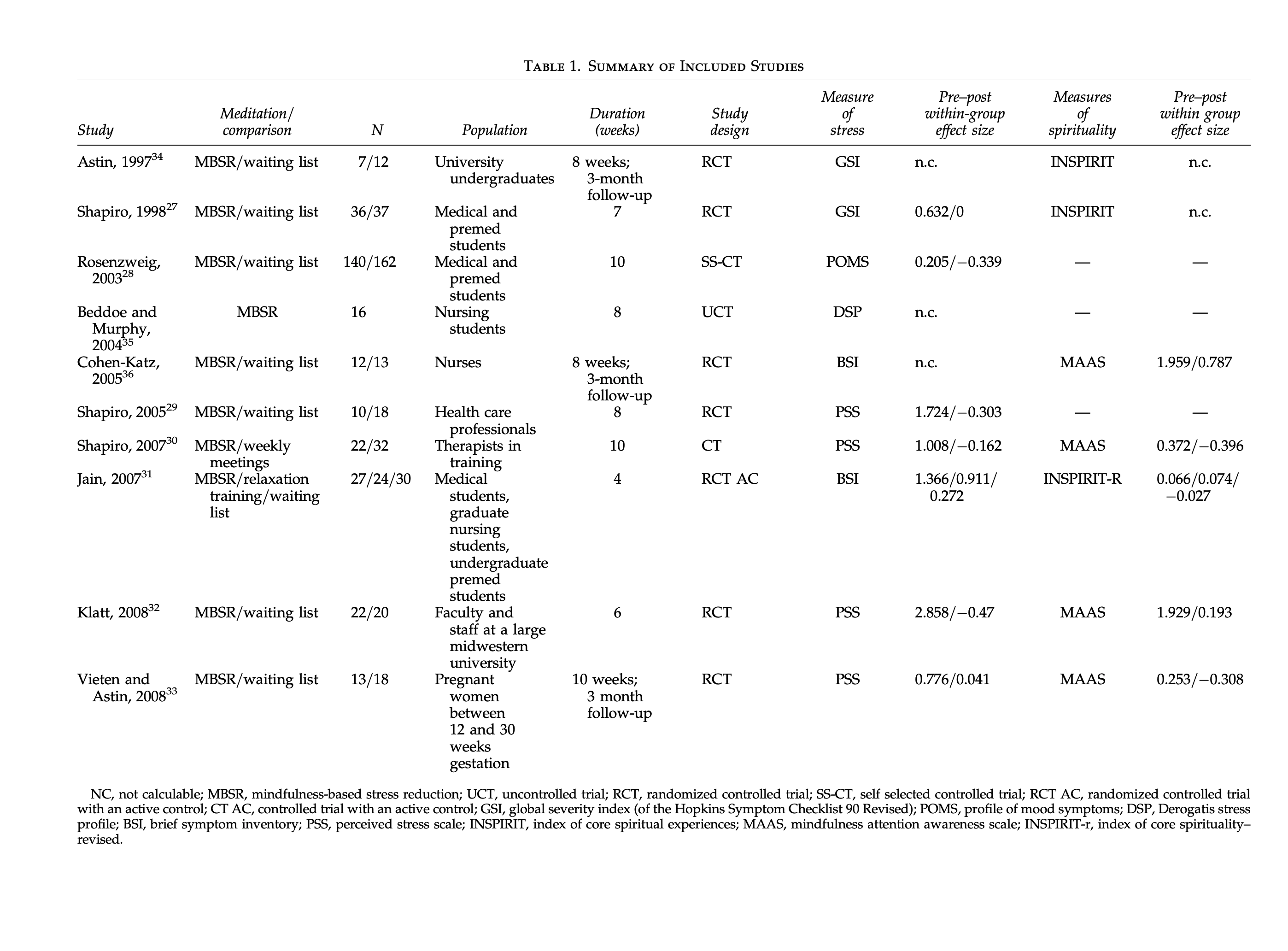
Within the table I am going to extract the study label study, the sample size for treatment (i.e., MBSR) and control (e.g., waitlist) group n_t and n_c, whether the study is an RCT (rct=1) or not (rct=0), the pre-post effect sizes for the both treatment (d_st_tx and d_sp_tx) and control (d_st_c and d_sp_c) groups for the stress and spiritual outcomes. Below is the final table in R:
Code
# data frame of original effects
df <- data.frame(
  study = c("Astin, 1997",
            "Shapiro, 1998",
            "Rosenzweig, 2003",
            "Beddoe and Murphy, 2004",
            "Cohen-Katz, 2005",
            "Shapiro, 2005",
            "Shapiro, 2007",
            "Jain, 2007",
            "Klatt, 2008",
            "Vieten and Astin, 2008"),
  d_st_tx=c(NA,0.632,0.205,NA,NA,1.724,1.008,1.366,2.858,0.776),
  d_st_c=c(NA,0.000,-0.339,NA,NA,-0.303, -0.162,0.272,-0.470,0.041),
  d_sp_tx= c(NA,NA,NA,NA,1.959,NA,0.372,0.066,1.929,0.253),
  d_sp_c= c(NA,NA,NA,NA,0.787,NA,-0.396,-0.027,0.193,-0.308),
  n_t= c(7,36,140, 16,12, 10,22,27,22,13),
  n_c= c(12,37,162,NA,13,18,32,30,20,18),
  rct=c(1,1,0,0,1,1,0,1,1,1))

head(df,10)
study d_st_tx d_st_c d_sp_tx d_sp_c n_t n_c rct
1 Astin, 1997 NA NA NA NA 7 12 1
2 Shapiro, 1998 0.632 0.000 NA NA 36 37 1
3 Rosenzweig, 2003 0.205 -0.339 NA NA 140 162 0
4 Beddoe and Murphy, 2004 NA NA NA NA 16 NA 0
5 Cohen-Katz, 2005 NA NA 1.959 0.787 12 13 1
6 Shapiro, 2005 1.724 -0.303 NA NA 10 18 1
7 Shapiro, 2007 1.008 -0.162 0.372 -0.396 22 32 0
8 Jain, 2007 1.366 0.272 0.066 -0.027 27 30 1
9 Klatt, 2008 2.858 -0.470 1.929 0.193 22 20 1
10 Vieten and Astin, 2008 0.776 0.041 0.253 -0.308 13 18 1Reproducing Data Extraction
In this section I look to reproduce the effect sizes from each of the studies in this table. At the end of this section I will have a summary table for my findings for all the studies. The function below will be used to calculate the pre-post effect sizes (per the equation reported by, Chiesa and Serretti 2009) from the study means and SDs.
d <- function(m1, s1, m2, s2, direction = "higher=better"){
  if (direction == "higher=better"){
   return((m2 - m1) / sqrt((s1^2 + s2^2)/2) )
  }

  if (direction == "higher=worse"){
    return(-1*(m2 - m1) / sqrt((s1^2 + s2^2)/2) )
  }
}
Reproducing: Astin (1997)
Chiesa and Serretti (2009) reported that the effects for both spiritual and stress outcomes in Astin (1997) were not calculable. Indeed the statistics reported in the paper were insufficient to calculate an exact effect without applying some strong assumptions. Though, it is important to point out that Astin (1997) showed a 64% reduction in stress (SCL-90) scores in the treatment group and a 14% reduction in the control group (see table below).
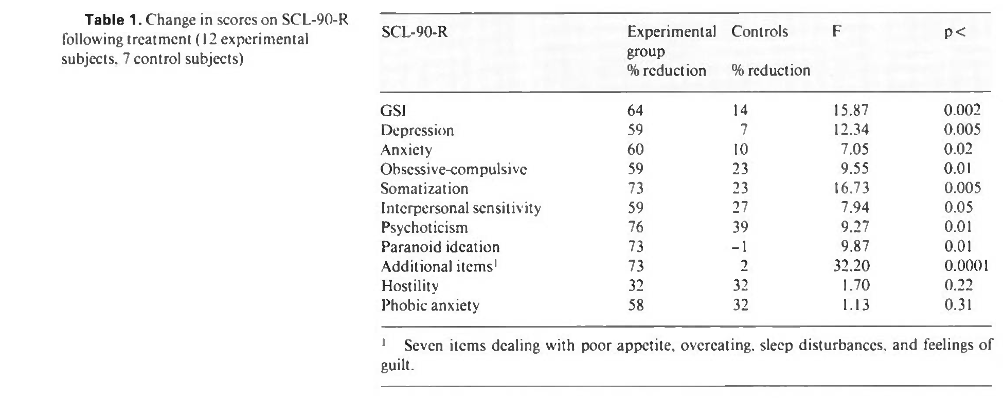
In the text, the same beneficial effect of the treatment is seen for the spirituality outcome (INSPIRIT), although again, there is not sufficient information to calculate an effect size.
Reproducing: Shapiro, Schwartz, and Bonner (1998)
The means and standard deviations (SDs) are located in Figure 1 of Shapiro, Schwartz, and Bonner (1998). Particularly panel d and e show the means and SDs for stress (measured by GSI) and spirituality, respectively. The stress figure is shown below below:
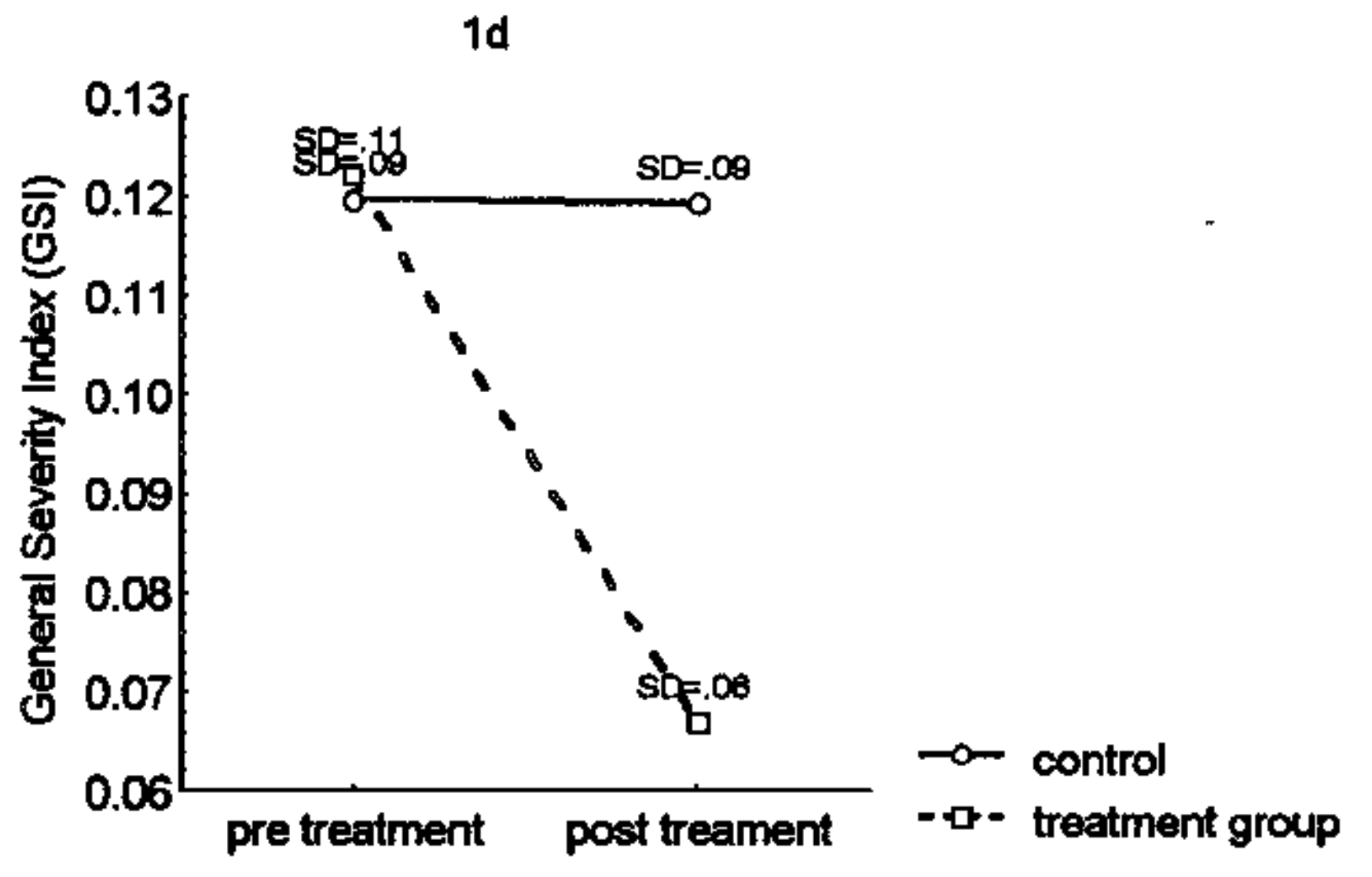
From the table the dots denote the mean and the SDs are labeled above them. For the post-treatment means, we observe a mean of .122 (SD = .11) for the treatment group and .120 (SD=.09) for the control group. For the pre-treatment means, we observe a mean of .066 (SD = .06) for the treatment group and .120 (SD=.09) for the control group. The effect size for stress will be as follows for both groups:
# treatment group (stress)
d(m1 = .122, s1 = .11,
  m2 = .066, s2 = .06,
  direction = "higher=worse")
[1] 0.6320526# control group (stress)
d(m1 = .120, s1 = .09,
m2 = .120, s2 = .09,
direction = "higher=worse")[1] 0The effect sizes match what is in Chiesa and Serretti (2009). For the spirituality effects, Chiesa and Serretti (2009) did not code the data and stated that it was “not calculable”, which appears to not be true since panel e has the spirituality data:
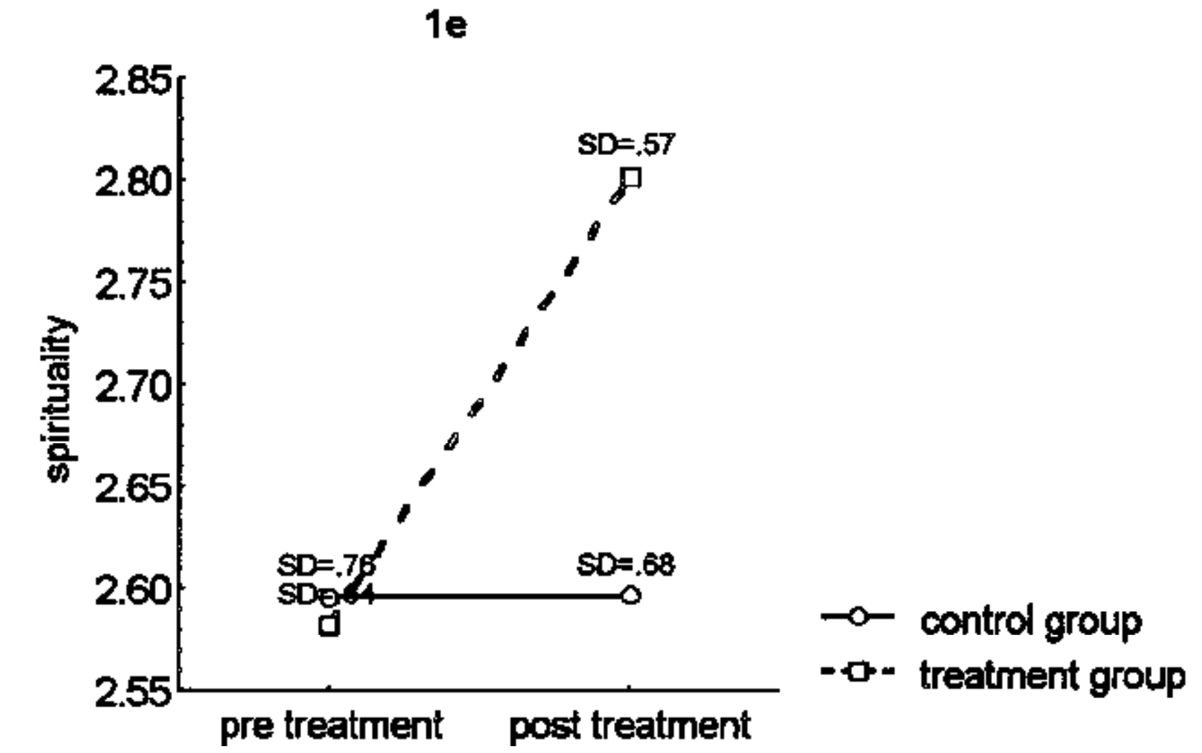
For the pre-treatment means, we observe a mean of 2.58 (SD = .64) for the treatment group and 2.59 (SD=.76) for the control group. For the post-treatment means, we observe a mean of 2.80 (SD = .57) for the treatment group and 2.59 (SD=.68) for the control group.
# treatment group (spirituality)
d(m1 = 2.58, s1 = .64,
  m2 = 2.80, s2 = .57,
  direction = "higher=better")
[1] 0.3630294# control group (spirituality)
d(m1 = 2.59, s1 = .76,
m2 = 2.59, s2 = .68,
direction = "higher=better")[1] 0This appears to be an error in the data extraction of the meta-analysis as I was able to successfully calculate the effect sizes for both treatment and control group for the spirituality outcome.
Reproducing: Rosenzweig et al. (2003)
Table 1 in Rosenzweig et al. (2003) reports the means and SDs for the Total Mood Disturbance index from the Profile of Mood States (POMS) scale which is used to measure stress:
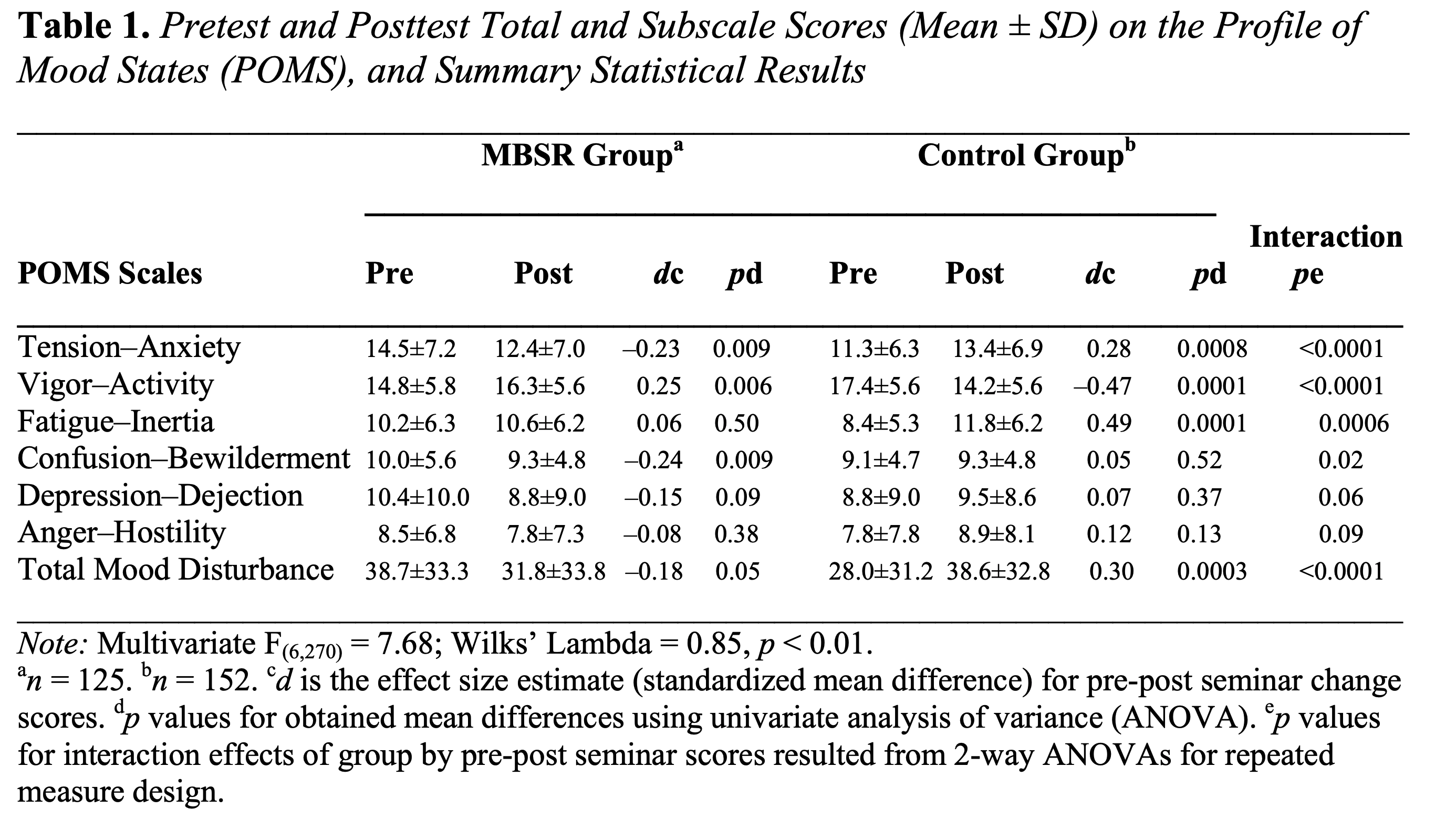
Using the Total Mood Disturbance score (i.e., POMS) we can see that for the pre-treatment means, we observe a mean of 38.7 (SD = 33.3) for the treatment group and 28.0 (SD=31.2) for the control group. For the post-treatment means, we observe a mean of 31.8 (SD = 33.8) for the treatment group and 38.6 (SD=32.8) for the control group. In R, let’s now calculate the effect.
# treatment group (stress)
d(m1 = 38.7, s1 = 33.3,
  m2 = 31.8, s2 = 33.8,
  direction = "higher=worse")
[1] 0.2056575# control group (stress)
d(m1 = 28.0, s1 = 31.2,
m2 = 38.6, s2 = 32.8,
direction = "higher=worse")[1] -0.3311465The effect sizes and the sample sizes (treatment group: d=.206, n=125; control group: d=–.331, n=152) are just slightly off from what is reported in Chiesa and Serretti (2009) (treatment group: d=.205, n=140; control group: d=–.331, n=162). Sample sizes appear to be extracted from the abstract, but that is the full sample, not the complete sample. In the table it is clear that these statistics are based on a sample size of 125 and 152 in the MBSR and control group, respectively.
Reproducing: Beddoe and Murphy (2004)
Chiesa and Serretti (2009) reported effects as incalculable. I am unable to gain access to this article so I am also unable to calculate any effects.
Reproducing: Cohen-Katz et al. (2005)
Chiesa and Serretti (2009) reported that the stress outcome was not calculable, however this is not the case. Cohen-Katz et al. (2005) measures stress from the BSI as a dichotomous variable (elevated stress vs not). Instead of continuous scores like we typically get from these outcomes, we can use the dichotomous scores to obtain an odds ratio and convert it to a Cohen’s d. We can observe the contingency table for pre-post comparisons as implied in the text on pages 31-32 of Cohen-Katz et al. (2005),
# treatment group
data.frame(stress = c("elevated","not elevated"),
           pre = c(3,9),
           post = c(1,11))
stress pre post
1 elevated 3 1
2 not elevated 9 11# control group
data.frame(stress = c("elevated","not elevated"),
pre = c(7,6),
post = c(4,9)) stress pre post
1 elevated 7 4
2 not elevated 6 9We can then calculate pre-post log odds ratios from the contingency tables and then convert to a Cohen’s d with the formula \(d = \frac{\log(OR)\times\sqrt{3}}{\pi}\),
# treatment group (flip so higher=better)
OR_tx <- (1/11)/(3/9)
d_tx <- (-1) * log(OR_tx)*sqrt(3)/pi
d_tx
[1] 0.7163323# control group (flip so higher=better)
OR_c <- (4/9)/(7/6)
d_c <- (-1) * log(OR_c)*sqrt(3)/pi
d_c[1] 0.532077I was therefore able to calculate the effect sizes for treatment and control for the stress outcomes.
The spirituality outcome effects are a bit harder. In Figure 2 of Cohen-Katz et al. (2005) below, they report the pre-post change for treatment and control group for the MAAS along with the p-value (presumably from the mean difference in change scores).
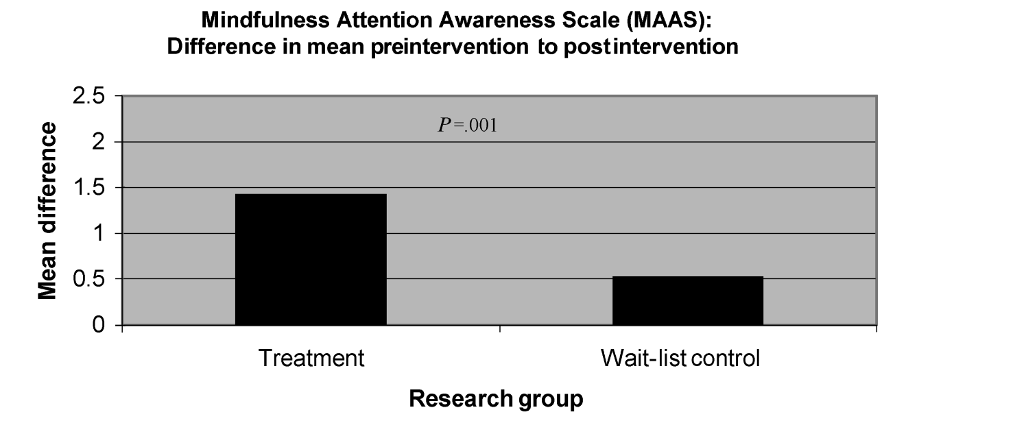
So for the effect sizes, we can start with getting the numerator (i.e., the raw mean change) from figure 2 where the mean change in the treatment group is about 1.4 and mean change in the control group is about 0.5. It is however unclear where the effect sizes of 1.959 and 0.787 come from since the pre and post-intervention standard deviations do not appear to be available. Instead, we will try to capture all possible effect size values based on the available information. The information that is available through the paper text and figures is the following:
- Treatment group:
- Pre-Intervention: Mean = 3, SD = unknown (from figure 3)
- Post-Intervention: Mean = 4.4, SD = unknown (from figure 2 and figure 3)
- pre-post correlation: r = unknown
- sample size: n = 12 (from page 29)
- Control Group:
- Pre-Intervention: Mean = Unknown, SD = unknown (from figure 3)
- Post-Intervention: Mean = pre-mean + 1.4, SD = unknown (from figure 2)
- pre-post correlation: r = unknown
- sample size: n = 13 (from page 29)
- Comparisons of Means:
- Pre-Pre (treatment vs control): p > .05 (implied from text on page 29)
- Post-Post (treatment vs control): p = .001 (from text on page 29)
- Pre-Post (treatment group): p = .004 (from figure 3)
Using the available information, we can attempt to construct a distribution of possible values for the pre-post effect size for the treatment and control group. For all unknown parameter values, we will draw parameter values from a uniform distribution over a plausible range of values. Using this space of parameters (known values are fixed and unknown values are randomly sampled), I will then generate 500,000 possible data sets and calculate the d value for treatment and control group for each one. Once the simulated d values are obtained, we will only select the ones from datasets that match the p-values reported in the text.
Code
# set seed and iteration count
set.seed(1)
iter = 500000

### randomly sampled unknown values ###
# standard deviations
s1_tx <- runif(iter,.5,2.5)
s2_tx <- runif(iter,.5,2.5)
s1_c <- runif(iter,.5,2.5)
s2_c <- runif(iter,.5,2.5)
# pre-post correlations
r_tx <- runif(iter,0,.999)
r_c <- runif(iter,0,.999)
m1_c <- runif(iter,1.5,4.5)

# known values
n_tx <- 12
n_c <- 13
m1_tx <- 3
m2_tx <- 4.4
m2_c <- m1_c + .5
p_tx = .004
p_post = .001
p_pre_thresh = .05 # non-significant threshold

# empty vector of p-values from simulations
p_tx_sim <- c()
p_post_sim <- c()
p_pre_sim <- c()

for(i in 1:iter){

  # generate pre-post data for treatment group
  df_tx <- mvrnorm(n_tx,
                  mu = c(m1_tx, m2_tx),
                  Sigma = data.frame(pre = c(s1_tx[i]^2, r_tx[i]*s1_tx[i]*s2_tx[i]),
                                     post = c(r_tx[i]*s1_tx[i]*s2_tx[i], s2_tx[i]^2)),
                  empirical = FALSE)

  # generate pre-post data for control group
  df_c <- mvrnorm(n_c,
                  mu = c(m1_c[i], m2_c[i]),
                  Sigma = data.frame(pre = c(s1_c[i]^2, r_c[i]*s1_c[i]*s2_c[i]),
                                     post = c(r_c[i]*s1_c[i]*s2_c[i], s2_c[i]^2)),
                  empirical = FALSE)

  # name pre and post columns
  colnames(df_tx) <- c("pre", "post")
  colnames(df_c) <- c("pre", "post")

  # p-values from simulated data
  p_tx_sim[i] <- t.test(df_tx[,"post"], df_tx[,"pre"], paired = TRUE)$p.value
  p_post_sim[i] <- t.test(df_tx[,"post"], df_c[,"post"], paired = FALSE)$p.value
  p_pre_sim[i] <- t.test(df_tx[,"pre"], df_c[,"pre"], paired = FALSE)$p.value

}

# get locations of p values within rounding error of .04
idx <- which(p_tx_sim > p_tx-.0005 & p_tx_sim < p_tx+.0005 &
             p_post_sim > p_post-.0005 & p_post_sim < p_post+.0005 &
             p_pre_sim > p_pre_thresh)

# calculate pre-post d treatment group
d_tx <- d(m1 = m1_tx, s1 = s1_tx[idx],
         m2 = m2_tx, s2 = s2_tx[idx],
         direction = "higher=better")

# calculate pre-post d in control group
d_c <- d(m1 = m1_c[idx], s1 = s1_c[idx],
         m2 = m2_c[idx], s2 = s2_c[idx],
         direction = "higher=better")

# save simulation
save(d_tx, d_c, file = "cohenkatz2005_simulation.RData")
Code
load("cohenkatz2005_simulation.RData")

# plot out possible values of d by treatment assignment
ggplot(data = NULL) +
  stat_slabinterval(aes(y = 0, x = d_c),point_interval = "mean_qi",
                    slab_fill = "grey50",slab_alpha = .5) +
  stat_slabinterval(aes(y = 1, x = d_tx),point_interval = "mean_qi",
                    slab_fill = "grey50",slab_alpha = .5) +
  geom_point(aes(x=0.787,y=0), color = "red3",size = 6, shape = 18) +
  geom_point(aes(x=1.959,y=1), color = "red3",size = 6, shape = 18) +
  geom_vline(xintercept = 0, linetype="dashed", alpha = .5) +
  scale_y_continuous(breaks = 0:1, labels = c("Control","Treatment"),limits = c(-.5,2)) +
labs(x = "Effect Size (d)", y = "") 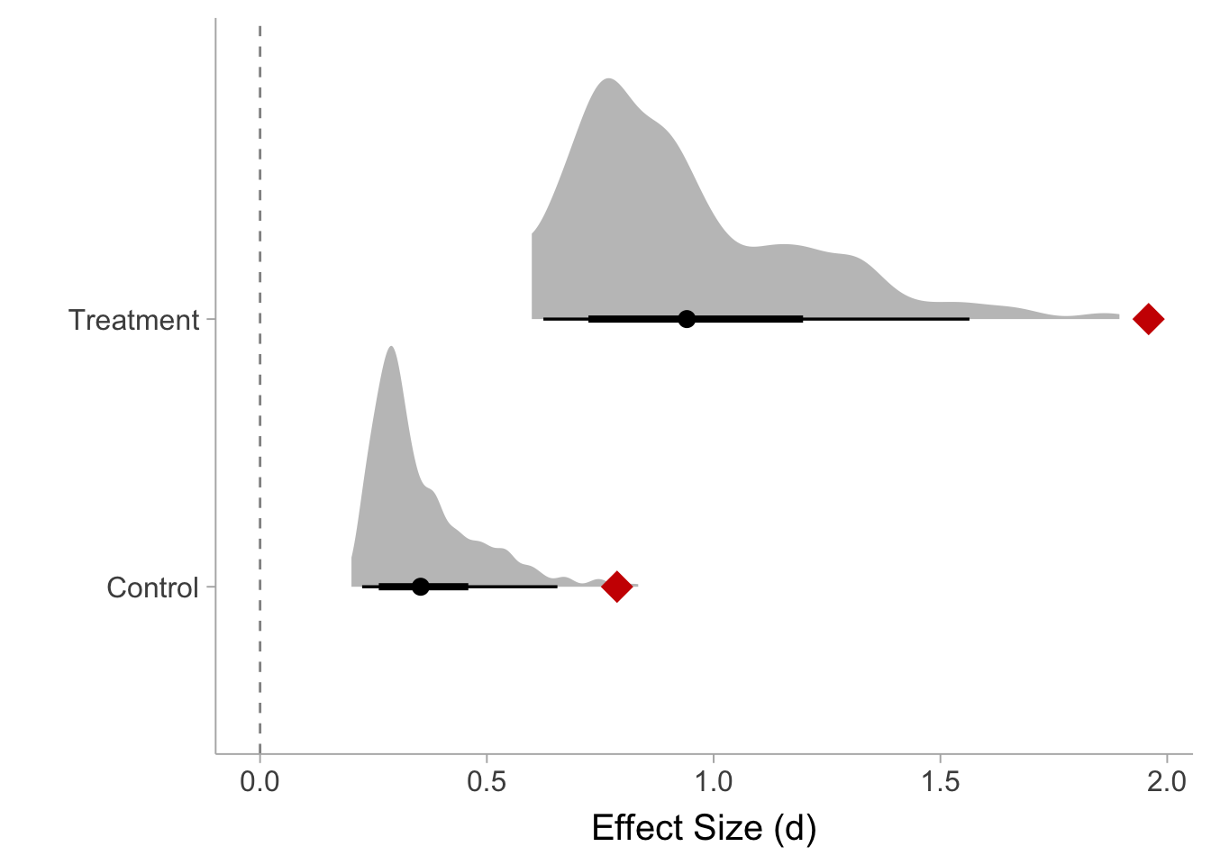
The effects reported by Chiesa and Serretti (2009) appear to be very unlikely according to the simulation. I will instead use the means of the two distributions as the approximate effect size for this study: d=.354 for the control group and d=.941 for the treatment group.
Reproducing: Shapiro et al. (2005)
The effect sizes reported by Chiesa and Serretti (2009) for Shapiro et al. (2005) are 1.724 and –.339 for the treatment and control group, respectively. However, in table 1 of Shapiro (2005), the treatment group and control group both reduce stress so it does not appear possible that the effect sizes are in different directions. Since Chiesa and Serretti (2009) ensures that beneficial effects of the treatment are positive, both the treatment and control group should see positive effects
Unfortunately, the study only reports means and no SDs and so it is unclear how the effects in Chiesa and Serretti (2009) are calculated. We have instead some information from a regression model that has the form \(\mathrm{stress_{post}} = \beta_0 + \beta_1\mathrm{stress_{pre}} + \beta_2 \mathrm{Tx}\), where \(\mathrm{Tx}\) denotes the dummy-coded treatment assignment. The p-value in the table is the p-value associated with the \(\beta_2\) coefficient. Similar to what we did with the previous section (see Reproducing: Cohen-Katz et al. 2005) we can simulate distributions of possible effect sizes based on the information provided in the table.
Code
# set seed and iteration count
set.seed(1)
iter = 10000

### randomly sampled unknown values ###
# standard deviations
s1_tx <- runif(iter,2,12)
s2_tx <- runif(iter,2,12)
s1_c <- runif(iter,2,12)
s2_c <- runif(iter,2,12)
# pre-post correlations
r_tx <- runif(iter,0,.999)
r_c <- runif(iter,0,.999)

# known values
n_tx <- 10
n_c <- 18
m1_tx <- 28.89
m2_tx <- 21.22
m1_c <- 23.78
m2_c <- 22.17
p = .04

# empty vector of p-values from simulations
psim <- c()

for(i in 1:iter){

  # generate pre-post data for treatment group
  df_tx <- mvrnorm(n_tx,
                  mu = c(m1_tx, m2_tx),
                  Sigma = data.frame(pre = c(s1_tx[i]^2, r_tx[i]*s1_tx[i]*s2_tx[i]),
                                     post = c(r_tx[i]*s1_tx[i]*s2_tx[i], s2_tx[i]^2)),
                  empirical = TRUE)

  # generate pre-post data for control group
  df_c <- mvrnorm(n_c,
                  mu = c(m1_c, m2_c),
                  Sigma = data.frame(pre = c(s1_c[i]^2, r_c[i]*s1_c[i]*s2_c[i]),
                                     post = c(r_c[i]*s1_c[i]*s2_c[i], s2_c[i]^2)),
                  empirical = TRUE)

  # concatenate treatment and control data
  df_total <- as.data.frame(rbind(df_tx,df_c))

  # name pre and post columns
  colnames(df_total) <- c("pre", "post")

  # create treatment assignment dummy code vector
  df_total <- cbind(df_total,
                    tx = c(rep(1,n_tx),rep(0,n_c)))

  # estimate regression model
  mdl <- lm(post ~ pre + tx, data = df_total)

  # extract p-value from treatment assignment term from model
  psim[i] <- coefficients(summary(lm(post ~ pre + tx,data = df_total)))[3,"Pr(>|t|)"]

}

# get locations of p values within rounding error of .04
idx <- which(psim > p-.005 & psim < p+.005)

# calculate pre-post d treatment group
d_tx <- d(m1 = m1_tx, s1 = s1_tx[idx],
         m2 = m2_tx, s2 = s2_tx[idx],
         direction = "higher=worse")

# calculate pre-post d in control group
d_c <- d(m1 = m1_c, s1 = s1_c[idx],
         m2 = m2_c, s2 = s2_c[idx],
         direction = "higher=worse")

# save simulation
save(d_tx, d_c, file = "shapiro2005_simulation.RData")
Code
load("shapiro2005_simulation.RData")

# plot out possible values of d by treatment assignment
ggplot(data = NULL) +
  stat_slabinterval(aes(y = 0, x = d_c),point_interval = "mean_qi",
                    slab_fill = "grey50",slab_alpha = .5) +
  stat_slabinterval(aes(y = 1, x = d_tx),point_interval = "mean_qi",
                    slab_fill = "grey50",slab_alpha = .5) +
  geom_point(aes(x=-.303,y=0), color = "red3",size = 6, shape = 18) +
  geom_point(aes(x=1.724,y=1), color = "red3",size = 6, shape = 18) +
  geom_vline(xintercept = 0, linetype="dashed", alpha = .5) +
  scale_y_continuous(breaks = 0:1, labels = c("Control","Treatment"),limits = c(-.5,2)) +
labs(x = "Effect Size (d)", y = "") 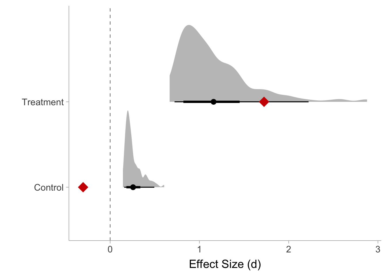
As expected, the reported effects by Chiesa and Serretti (2009) are impossible for the control group, but it may be possible for the treatment group. It is quite possible that Chiesa and Serretti (2009) simply coded the wrong direction for the control group, but it is still unclear how the effects are calculated as the paper does provide the necessary information. Due to the inability to reproduce Chiesa and Serretti (2009)’s results, I will use the mean of the simulated effect sizes instead: 1.159 for the treatment group and .257 for the control group.
Reproducing: Shapiro, Brown, and Biegel (2007)
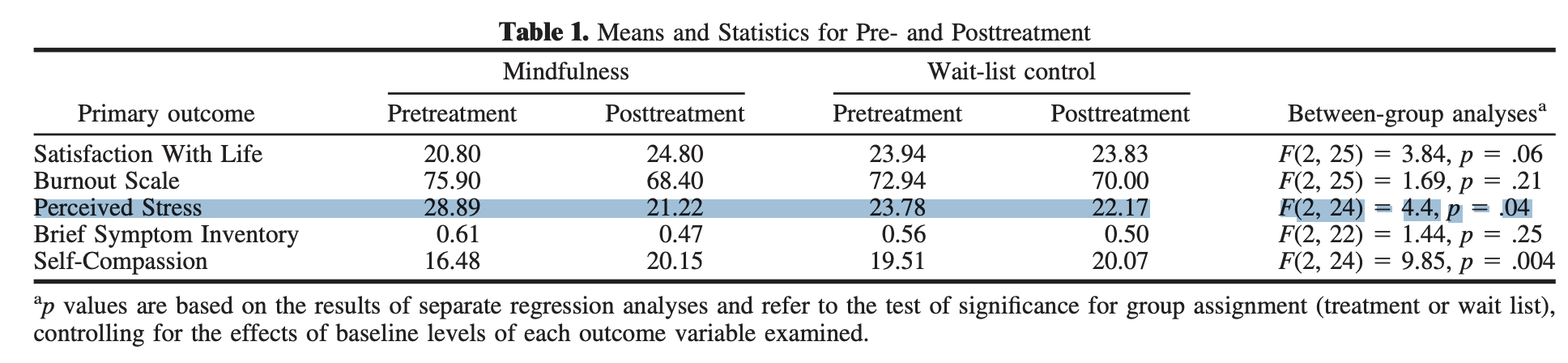
Chiesa and Serretti (2009) reported the stress pre-post effect sizes for Shapiro, Brown, and Biegel (2007) as follows 1.008 and –.162 for the treatment and control group, respectively. Chiesa and Serretti (2009) then reported the spirituality effect sizes as .372 and –.396 for treatment and control group, respectively. Table 1 of Shapiro, Brown, and Biegel (2007) has all the necessary information to calculate effect sizes:
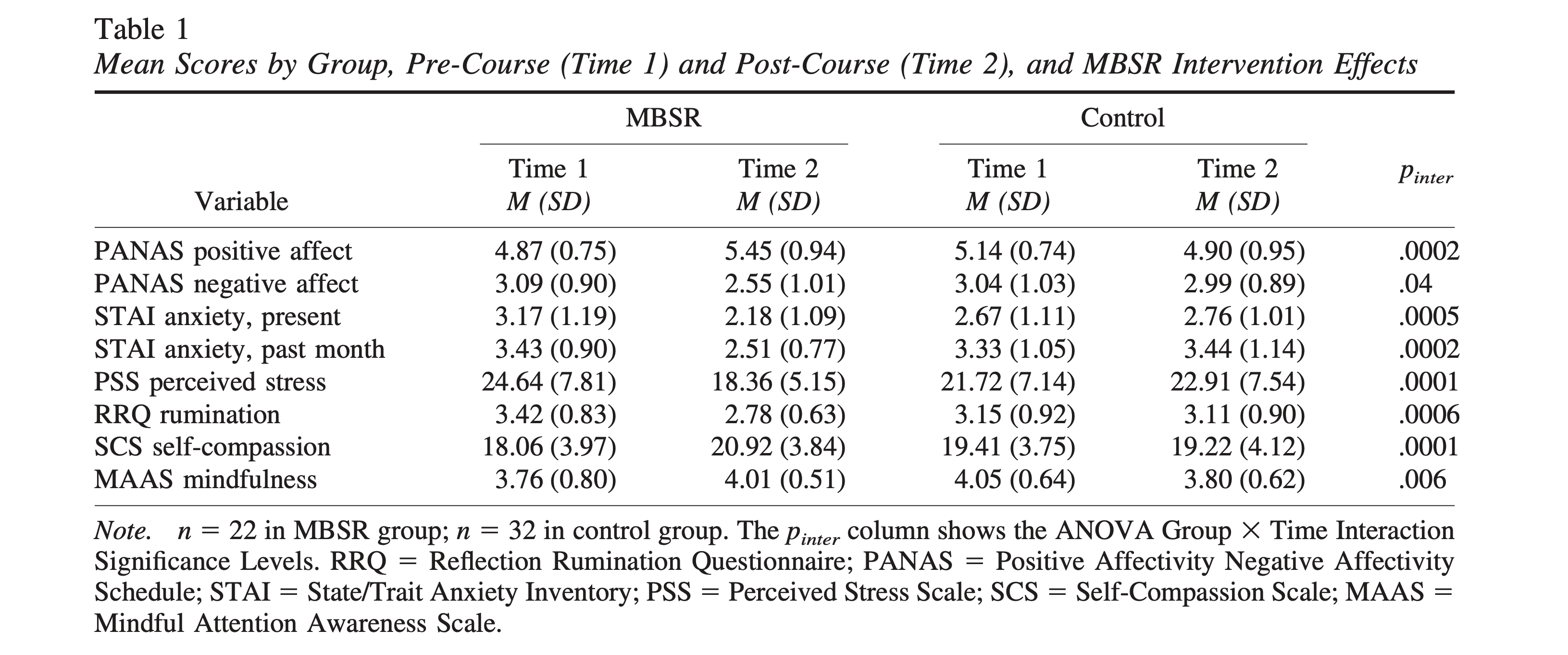
From this table we can extract the statistics and calculate the pre-post effect sizes for the stress outcome (Perceived Stress Scale, PSS) and the spirituality outcome (Mindful Attention Awareness Scale, MAAS):
## STRESS
data.frame(
  # treatment group
  d_treatment = d(m1 = 24.64, s1 = 7.81,
                  m2 = 18.36, s2 = 5.15,
                  direction = "higher=worse"),
  # control group
  d_control = d(m1 = 21.72, s1 = 7.14,
                m2 = 22.91, s2 = 7.54,
                direction = "higher=worse")
)
d_treatment d_control
1 0.9493459 -0.1620652## SPIRITUALITY
data.frame(
# treatment group
d_treatment = d(m1 = 3.76, s1 = 0.80,
m2 = 4.01, s2 = 0.51,
direction = "higher=better"),
# control group
d_control = d(m1 = 4.05, s1 = 0.64,
m2 = 3.80, s2 = 0.62,
direction = "higher=better")
) d_treatment d_control
1 0.3726573 -0.3967754The effects from Chiesa and Serretti (2009) were mostly reproducible within rounding error, however, the treatment group in the stress outcome was a bit off (Chiesa reported 1.008, but my calculation shows .949). From what I can tell, this is due to a simple data copying error. When I use SD=7.15 instead of 7.81 in the pre-test I recover the 1.008 effect that Chiesa and Serretti (2009) reported (the post-test value also ends in the decimal 5.15 which makes it appear to be a simple copy and paste mistake).
Reproducing: Jain et al. (2007)
Jain et al. (2007) has three intervention arms: a control, relaxation group, and a meditation group (the treatment). Jain et al. (2007) also had a measure of stress (Brief Symptom Inventory, BSI) and a measure of spirituality (Index of Core Spiritual Experiences). Chiesa and Serretti (2009) reported the effects for the stress outcome as 1.366 for the meditation (treatment) group, .911 for the relaxation group and .272 for the control group. As for the spirituality outcome, Chiesa and Serretti (2009) reported .066 for the meditation (treatment) group, .074 for the relaxation group and -.027 for the control group. Table 1 of Jain et al. (2007) contains the necessary statistics to calculate the effect sizes:
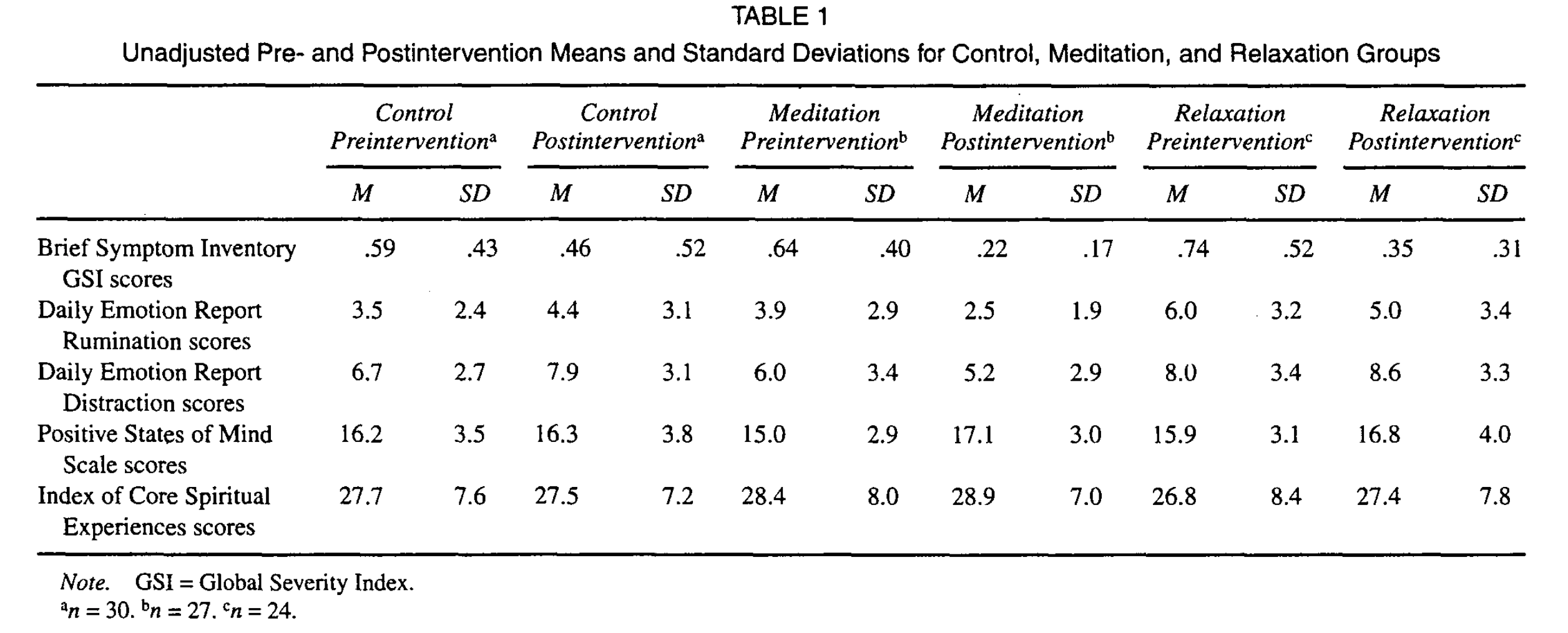
We can then extract the means and SDs and calculate the pre-post effect sizes for each group.
## STRESS
data.frame(
  # meditation (treatment) group
  d_treatment = d(m1 = .64, s1 = .40,
                  m2 = .22, s2 = .17,
                  direction = "higher=worse"),
  # relaxation group
  d_relaxation = d(m1 = .74, s1 = .52,
                m2 = .35, s2 = .31,
                direction = "higher=worse"),
  # control group
  d_control = d(m1 = .59, s1 = .43,
                m2 = .46, s2 = .52,
                direction = "higher=worse")
)
d_treatment d_relaxation d_control
1 1.366622 0.9110508 0.2724642## SPIRITUALITY
data.frame(
# meditation (treatment) group
d_treatment = d(m1 = 28.4, s1 = 8,
m2 = 28.9, s2 = 7,
direction = "higher=better"),
# relaxation group
d_relaxation = d(m1 = 26.8, s1 = 8.4,
m2 = 27.4, s2 = 7.8,
direction = "higher=better"),
# control group
d_control = d(m1 = 27.7, s1 = 7.6,
m2 = 27.5, s2 = 7.2,
direction = "higher=better")
) d_treatment d_relaxation d_control
1 0.06651901 0.07402332 -0.02701716I was able to exactly reproduce the effect sizes that were calculated by Chiesa and Serretti (2009).
Reproducing: Klatt, Buckworth, and Malarkey (2009)
Chiesa and Serretti (2009) reported the effect sizes for the stress outcome (Perceived Stress Scale, PSS) was 2.858 and –0.47 for the treatment and control group, respectively. They also reported for the spirituality outcome (Mindful Attention Awareness Scale, MAAS) as 1.929 and 0.193 for the treatment and control group, respectively. The statistics needed to calculate the pre-post effect sizes are found in table 2 of Klatt, Buckworth, and Malarkey (2009):
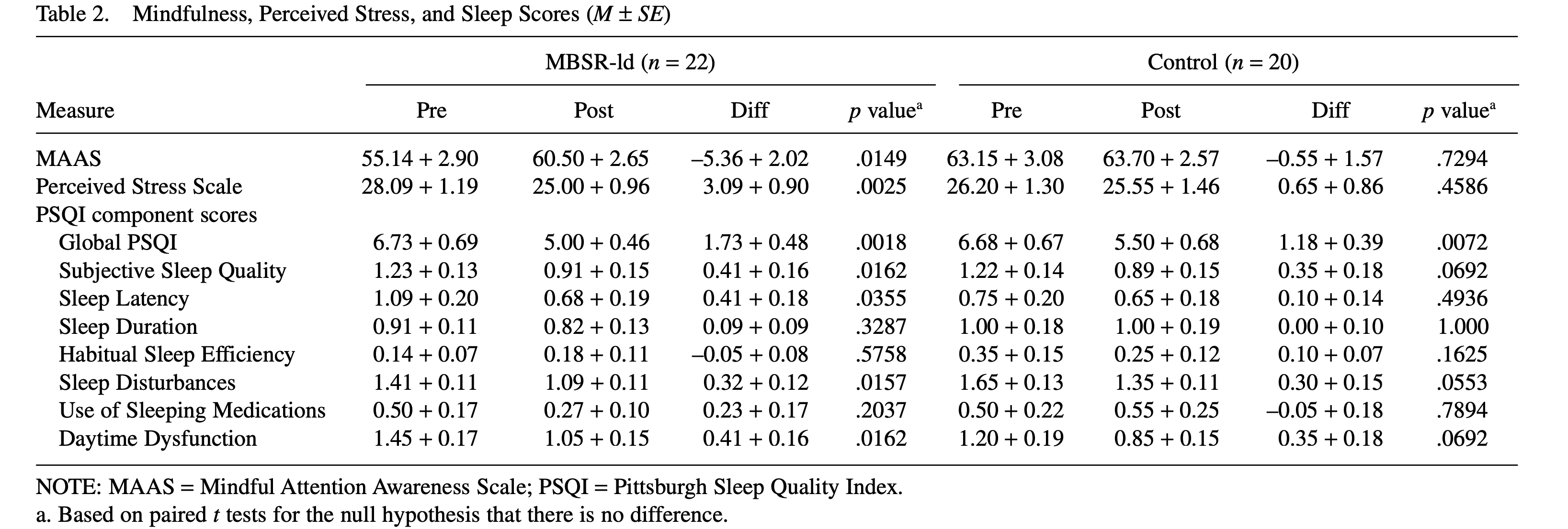
According to the caption, the descriptive statistics are reported as \(\textrm{Mean} \pm \textrm{SE}\) where SE denotes the standard error of the mean. Before we can calculate the effect size, we have to convert the standard errors to standard deviation which we can do simply by multiplying it by the square root of the sample size, \(SD=SE\times\sqrt{n}\). It appears that Chiesa and Serretti (2009) skipped that step and instead used the standard errors as standard deviations in the effect size formula, that has the consequence of greatly inflating the effect size as we will see. Let’s calculate the effect sizes properly and then try to also reproduce Chiesa and Serretti (2009)’s effect size calculation:
# sample sizes for control (c) and treatment (tx) group
n_c <- 20
n_tx <- 22

## STRESS
data.frame(
  # treatment group
  d_treatment = d(m1 = 28.09, s1 = 1.19*sqrt(n_tx),
                  m2 = 25.00, s2 = 0.96*sqrt(n_tx),
                  direction = "higher=worse"),
  # control group
  d_control = d(m1 = 26.20, s1 = 1.30*sqrt(n_c),
                m2 = 25.55, s2 = 1.46*sqrt(n_c),
                direction = "higher=worse")
)
d_treatment d_control
1 0.6093513 0.1051455## SPIRITUALITY
data.frame(
# treatment group
d_treatment = d(m1 = 55.14, s1 = 2.90*sqrt(n_tx),
m2 = 60.50, s2 = 2.65*sqrt(n_tx),
direction = "higher=better"),
# control group
d_control = d(m1 = 63.15, s1 = 3.08*sqrt(n_c),
m2 = 63.70, s2 = 2.57*sqrt(n_c),
direction = "higher=better")
) d_treatment d_control
1 0.4113868 0.04335779It’s clear that the effect sizes are much smaller than what is reported in Chiesa and Serretti (2009). We can try to reproduce Chiesa and Serretti (2009)’s reported effects by using the standard error instead of the standard deviation when calculating the effect sizes:
## STRESS
data.frame(
  # treatment group
  d_treatment = d(m1 = 28.09, s1 = 1.19,
                  m2 = 25.00, s2 = 0.96,
                  direction = "higher=worse"),
  # control group
  d_control = d(m1 = 26.20, s1 = 1.30,
                m2 = 25.55, s2 = 1.46,
                direction = "higher=worse")
)
d_treatment d_control
1 2.858111 0.470225## SPIRITUALITY
data.frame(
# treatment group
d_treatment = d(m1 = 55.14, s1 = 2.90,
m2 = 60.50, s2 = 2.65,
direction = "higher=better"),
# control group
d_control = d(m1 = 63.15, s1 = 3.08,
m2 = 63.70, s2 = 2.57,
direction = "higher=better")
) d_treatment d_control
1 1.929575 0.1939019I was able to reproduce the values reported by Chiesa and Serretti (2009) when improperly calculating the effect size using the standard errors. However, there is also a mistake in the direction of the effect size for the control group in the stress outcome. Chiesa and Serretti (2009) report negative pre-post effect in the control group even though stress decreased for both groups and therefore both effects should be positive.
Reproducing: Vieten and Astin (2008)
Chiesa and Serretti (2009) reported the stress outcome (Perceived Stress Scale, PSS) pre-post effect sizes for Vieten and Astin (2008) as 0.776 and 0.041 for the treatment and control group, respectively. Chiesa and Serretti (2009) then reported the spirituality outcome (Mindful Attention Awareness Scale, MAAS) effect sizes as 0.253 and –0.308 for treatment and control group, respectively. Table 1 from Vieten and Astin (2008) provides the information necessary to calculate the pre-post effects:
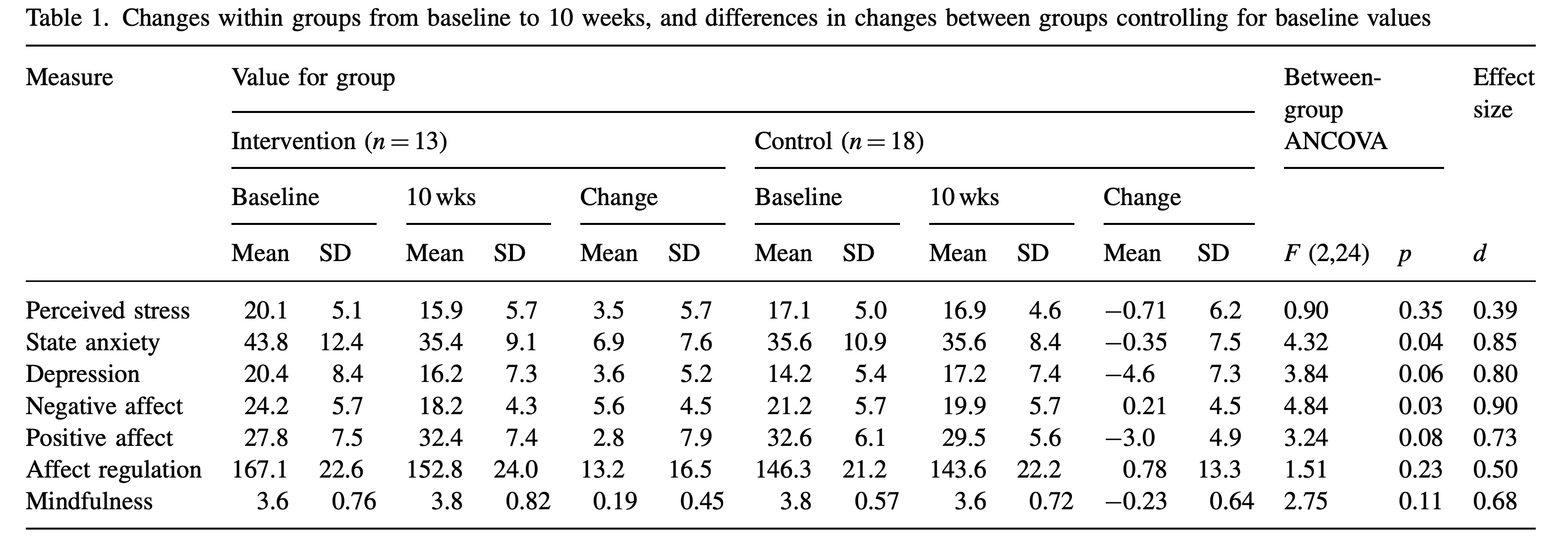
This table has some strange anomolies such as the change score means not being equal to the difference in pre and post-test means (e.g., for stress in the intervention group \(15.9-20.1\neq 3.5\)). Also, the F-statistics with \(F(2,24)\) does not produce the p-values reported in the paper (e.g., for stress if \(F(2,24) = .90\) then \(p =0.4199\)). The statistics as they are reported are likely untrustworthy In R, let’s calculate the effect sizes from the table:
## STRESS
data.frame(
  # treatment group
  d_treatment = d(m1 = 20.1, s1 = 5.1,
                  m2 = 15.8, s2 = 5.7,
                  direction = "higher=worse"),
  # control group
  d_control = d(m1 = 17.1, s1 = 5.0,
                m2 = 16.9, s2 = 4.6,
                direction = "higher=worse")
)
d_treatment d_control
1 0.7950703 0.04163054## SPIRITUALITY
data.frame(
# treatment group
d_treatment = d(m1 = 3.6, s1 = 0.76,
m2 = 3.8, s2 = 0.82,
direction = "higher=better"),
# control group
d_control = d(m1 = 3.8, s1 = 0.57,
m2 = 3.6, s2 = 0.72,
direction = "higher=better")
) d_treatment d_control
1 0.2529822 -0.3080023There is only a slight discrepency in the stress outcome where Chiesa and Serretti (2009)’s reported effect was .776 for the treatment group and I calculated .795. Otherwise the effects were reproducible.
Summarizing and visualizing the errors
I highlighted and annotated the corrections in table 1 of Chiesa and Serretti (2009). The edited table below shows three types of errors
- insufficient information/implausible results: effect sizes are not calculable directly from what is reported in the study. Effect sizes were then calculated by simulating plausible data sets from the available information. Then it is determined whether the effects reported by Chiesa and Serretti (2009) are plausible, if not, the mean of the simulated effect sizes will be the effect for that study.
- major error: corrected effect sizes are off by more than \(\pm.05\).
- minor error: corrected effect sizes are off by less than \(\pm.05\). Also minor errors will include sample size errors (there was only one).
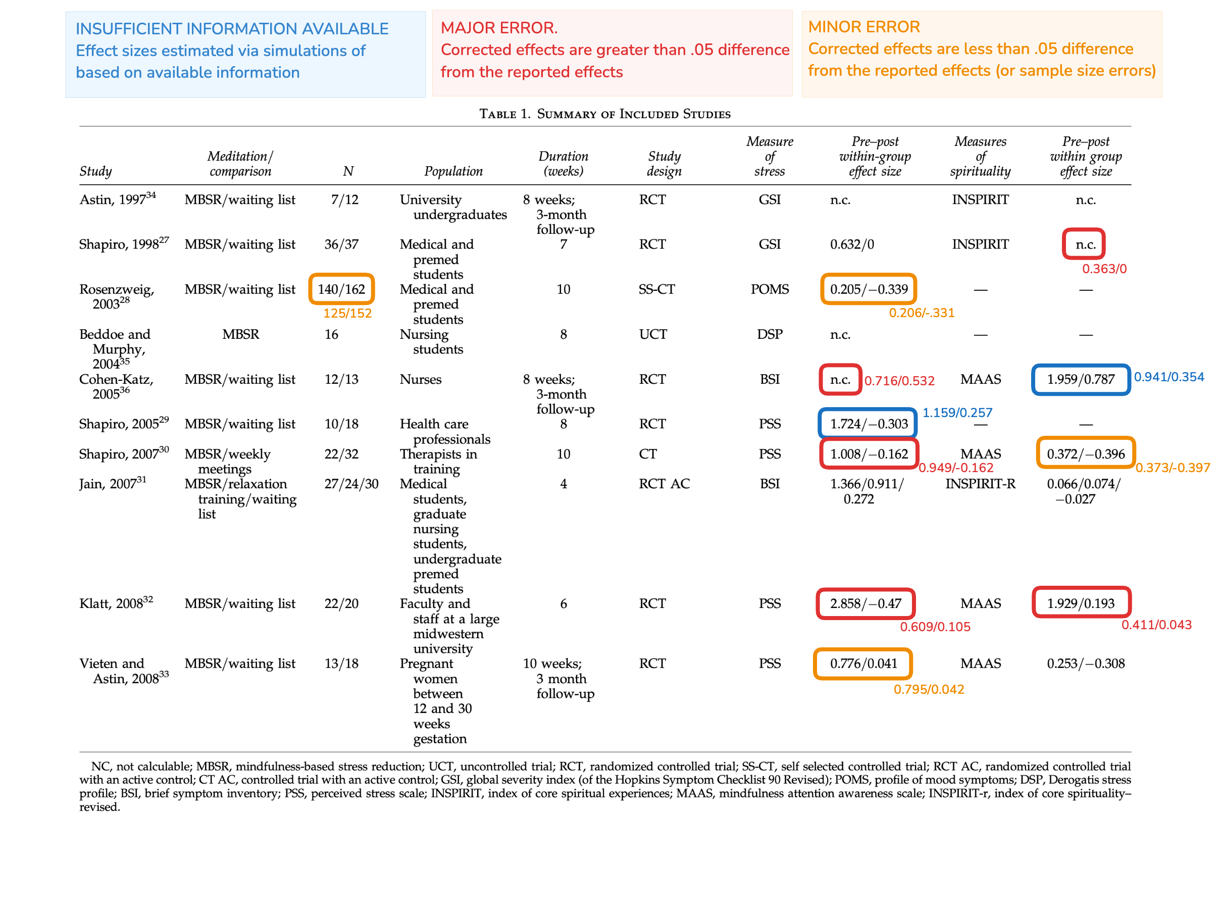
For 10 studies that had stress outcomes, there were 3 major errors, 2 minor errors, and 1 study with insufficient information/implausible results. For 7 studies that had spirituality outcomes, there were 2 major errors, 1 minor error, and 1 study with insufficient information/implausible results. We can append the data frame constructed at the beginning of the report with the corrected values (denoted with corr suffix):
df <- df %>%
  mutate(d_st_tx_corr = c(NA,.632, .206,NA,.716,1.159,.949, 1.366,.609,.795),
         d_st_c_corr =  c(NA,   0,-.331,NA,.532, .257,-.162, .272, .105,.042),
         d_sp_tx_corr = c(NA,.363,NA,NA,.941,NA,.373,.066,.411,.253),
         d_sp_c_corr =  c(NA,0,NA,NA,.354,NA,-.396,-.027,.193,-.308),
         n_t_corr = c(7,36,125, 16,12, 10,22,27,22,13),
         n_c_corr = c(12,37,152,NA,13,18,32,30,20,18))
The figures below shows the differences between treatment and control group \(\Delta=d_\mathrm{Tx} - d_\mathrm{C}\). Figure 1 shows all the studies with stress outcomes where the circles denote the effect differences \(\Delta\) and the diamond denotes the sample size weighted mean of \(\Delta\).
Code
set.seed(1)
library(patchwork)

h_st <- ggplot(data = df) +
  geom_jitter(aes(x = d_st_tx_corr, y = 1, size = n_t),
              height = .2, width = 0, alpha = .4) +
  geom_jitter(aes(x = d_st_tx, y = 0,size = n_t),
              height = .2, width = 0, alpha = .4) +
  geom_point(aes(x = weighted.mean(d_st_tx_corr - d_st_c_corr, n_t_corr+n_c_corr,na.rm=T),
                 y = 1),
             size = 7,color = "black", shape = 18) +
  geom_point(aes(x = weighted.mean(d_st_tx - d_st_c, n_t+n_c,na.rm=T),
                 y = 0),
             size = 7,color = "black", shape = 18) +
  theme(aspect.ratio = .4, legend.position = "none") +
  geom_vline(xintercept = 0, linetype = "dashed") +
  geom_vline(xintercept = seq(.25,3,by=.25),
             linetype = "dashed",alpha=.07) +
  scale_y_continuous(breaks = 0:1,
                     labels = c("Reported", "Corrected"),
                     limits = c(-.5,1.5)) +
  scale_x_continuous(breaks = 0:6/2) +
  labs(x = "",
       y = "",
       title = "All studies (Stress)")


hrct_st <- ggplot(data = df %>% filter(rct == 1)) +
  geom_jitter(aes(x = d_st_tx_corr, y = 1, size = n_t),
              height = .2, width = 0, alpha = .4) +
  geom_jitter(aes(x = d_st_tx, y = 0,size = n_t),
              height = .2, width = 0, alpha = .4) +
  geom_point(aes(x = weighted.mean(d_st_tx_corr - d_st_c_corr, n_t_corr+n_c_corr,na.rm=T),
                 y = 1),
             size = 7,color = "black", shape = 18) +
  geom_point(aes(x = weighted.mean(d_st_tx - d_st_c, n_t+n_c,na.rm=T),
                 y = 0),
             size = 7,color = "black", shape = 18) +
  theme(aspect.ratio = .4, legend.position = "none") +
  geom_vline(xintercept = 0, linetype = "dashed") +
  geom_vline(xintercept = seq(.25,3,by=.25), linetype = "dashed",alpha=.07) +
  scale_y_continuous(breaks = 0:1,
                     labels = c("Reported", "Corrected"),
                     limits = c(-.5,1.5)) +
  scale_x_continuous(breaks = 0:6/2) +
  labs(x = "Treatment-Control Diff in Effects (Δ)",
       y = "",
       title = "RCTs Only (Stress)")

h_st / hrct_st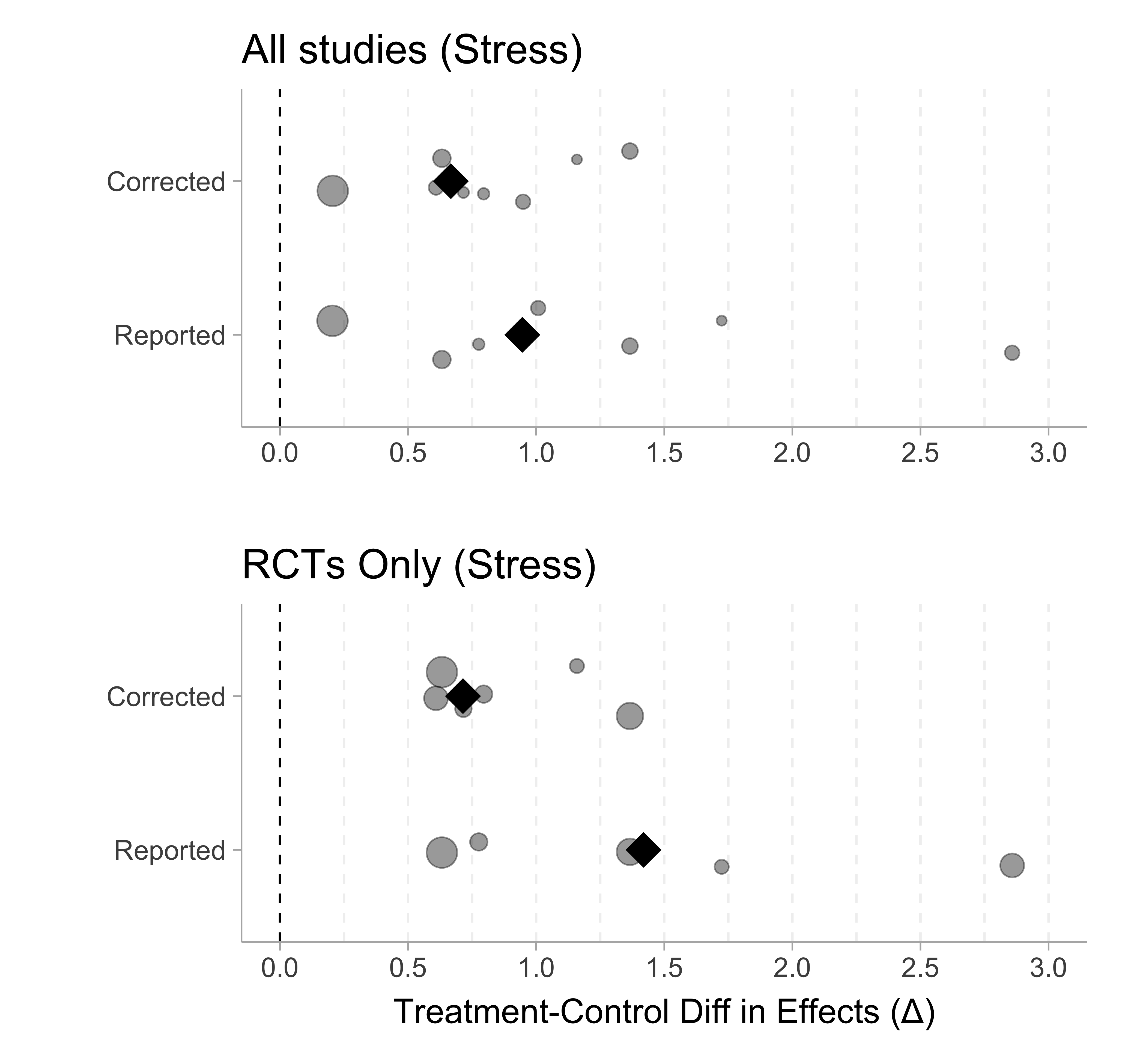
Figure 1 shows the spirituality outcome where the circles denote the study effect differences and the diamond denotes the sample size weighted mean.
Code
set.seed(1)

h_sp <- ggplot(data = df) +
  geom_jitter(aes(x = d_sp_tx_corr, y = 1, size = n_t),
              height = .2, width = 0, alpha = .4) +
  geom_jitter(aes(x = d_sp_tx, y = 0,size = n_t),
              height = .2, width = 0, alpha = .4) +
  geom_point(aes(x = weighted.mean(d_sp_tx_corr-d_sp_c_corr, n_t_corr+n_c_corr,na.rm=T),
                 y = 1),
             size = 7,color = "black", shape = 18) +
  geom_point(aes(x = weighted.mean(d_sp_tx-d_sp_c, n_t+n_c,na.rm=T),
                 y = 0),
             size = 7,color = "black", shape = 18) +
  theme(aspect.ratio = .4, legend.position = "none") +
  geom_vline(xintercept = 0, linetype = "dashed") +
  geom_vline(xintercept = seq(.25,3,by=.25),
             linetype = "dashed",alpha=.07) +
  scale_y_continuous(breaks = 0:1,
                     labels = c("Reported", "Corrected"),
                     limits = c(-.5,1.5)) +
  scale_x_continuous(breaks = 0:6/2) +
  labs(x = "",
       y = "",
       title = "All studies (Spirituality)")


hrct_sp <- ggplot(data = df %>% filter(rct == 1)) +
  geom_jitter(aes(x = d_sp_tx_corr, y = 1, size = n_t),
              height = .2, width = 0, alpha = .4) +
  geom_jitter(aes(x = d_sp_tx, y = 0,size = n_t),
              height = .2, width = 0, alpha = .4) +
  geom_point(aes(x = weighted.mean(d_sp_tx_corr-d_sp_c_corr, n_t_corr+n_c_corr,na.rm=T),
                 y = 1),
             size = 7,color = "black", shape = 18) +
  geom_point(aes(x = weighted.mean(d_sp_tx-d_sp_c, n_t+n_c,na.rm=T),
                 y = 0),
             size = 7,color = "black", shape = 18) +
  theme(aspect.ratio = .4, legend.position = "none") +
  geom_vline(xintercept = 0, linetype = "dashed") +
  geom_vline(xintercept = seq(.25,3,by=.25), linetype = "dashed",alpha=.07) +
  scale_y_continuous(breaks = 0:1,
                     labels = c("Reported", "Corrected"),
                     limits = c(-.5,1.5)) +
  scale_x_continuous(breaks = 0:6/2) +
  labs(x = "Treatment-Control Diff in Effects (Δ)",
       y = "",
       title = "RCTs Only (Spirituality)")

h_sp / hrct_sp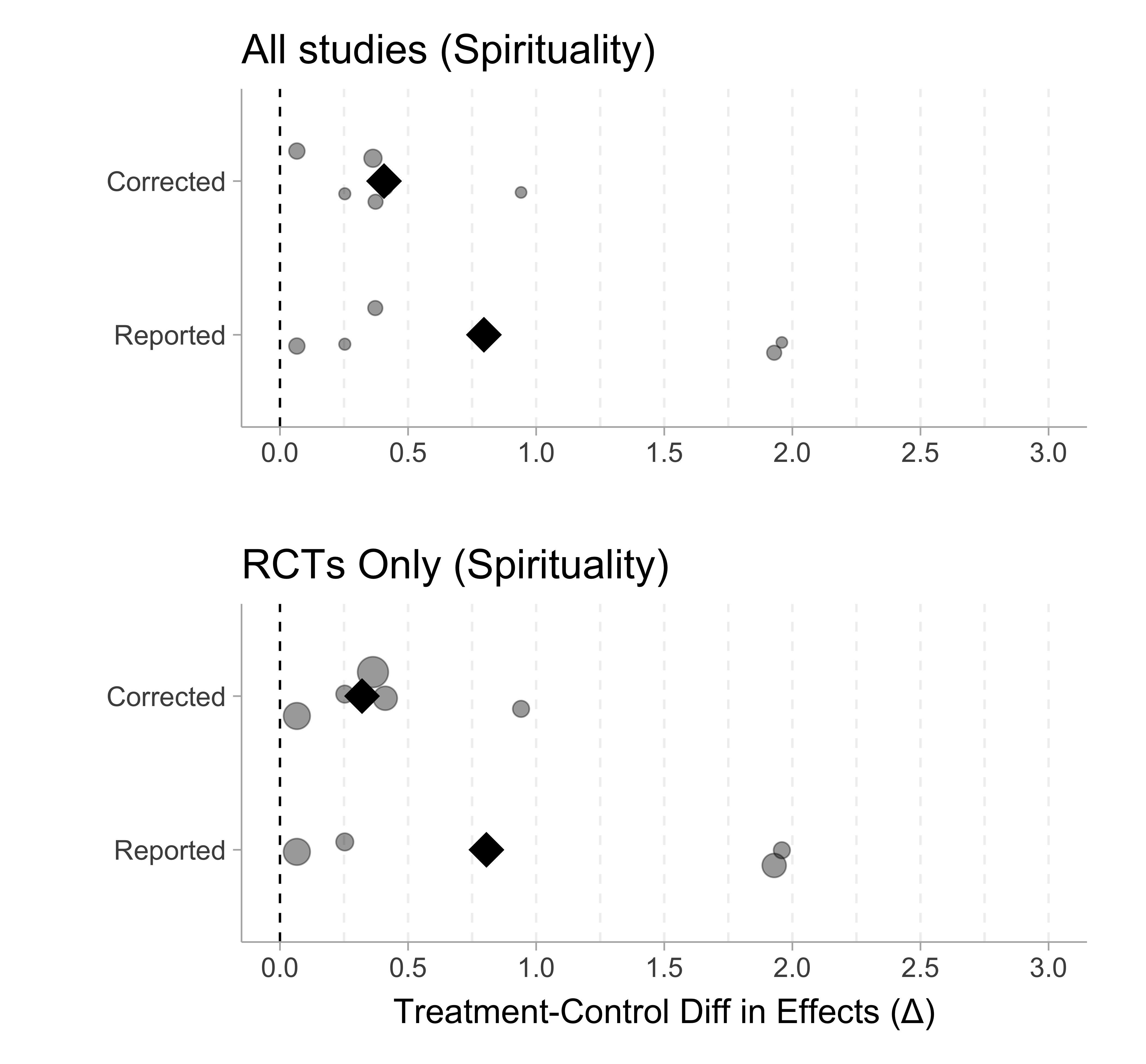
As we can see from both Figure 1 and Figure 2, the reported treatment-control difference is substantially larger than the corrected effect sizes for both the stress and spirituality outcomes. This suggests the results reported in Chiesa and Serretti (2009) are artificially large.
Analysis Flaws
Chiesa and Serretti (2009) uses an N-weighted t-test to analyze the contrast between treatment and control pre-post effect sizes. This is an inappropriate statistical method for meta-analysis for two reasons: it does not properly model the heterogeneity in effects and it treats effects as fixed rather than estimated values. The method employed by Chiesa and Serretti (2009) artificially shrinks the standard errors (and thus confidence intervals) of average effects. A standard meta-analysis uses random-effects weights and estimation to calculate the mean and confidence interval of the mean effect size across studies (see the Cochrane handbook https://training.cochrane.org/handbook/current/chapter-10#section-10-10-4).
Instead of comparing the means of pre-post effects independently, they should be modeled jointly since treatment and control pre-post effects coming from the same study tend to be correlated (e.g., for stress, we see a correlation of r=.52).
Conclusion
Due to the severe data extraction errors and analysis flaws, the primary meta-analytic results in table 4 in Chiesa and Serretti (2009) are incorrect and greatly exaggerate the effect between treatment and control groups for both stress and spirituality outcomes.
References
Astin, John A. 1997. “Stress Reduction Through Mindfulness Meditation: Effects on Psychological Symptomatology, Sense of Control, and Spiritual Experiences.” Psychotherapy and Psychosomatics 66 (2): 97–106.
Beddoe, Amy E, and Susan O Murphy. 2004. “Does Mindfulness Decrease Stress and Foster Empathy Among Nursing Students?” Journal of Nursing Education 43 (7): 305–12.
Chiesa, Alberto, and Alessandro Serretti. 2009. “Mindfulness-Based Stress Reduction for Stress Management in Healthy People: A Review and Meta-Analysis.” The Journal of Alternative and Complementary Medicine 15 (5): 593–600.
Cohen-Katz, Joanne, Susan D Wiley, Terry Capuano, Debra M Baker, and Shauna Shapiro. 2005. “The Effects of Mindfulness-Based Stress Reduction on Nurse Stress and Burnout, Part II: A Quantitative and Qualitative Study.” Holistic Nursing Practice 19 (1): 26–35.
Jain, Shamini, Shauna L Shapiro, Summer Swanick, Scott C Roesch, Paul J Mills, Iris Bell, and Gary ER Schwartz. 2007. “A Randomized Controlled Trial of Mindfulness Meditation Versus Relaxation Training: Effects on Distress, Positive States of Mind, Rumination, and Distraction.” Annals of Behavioral Medicine 33: 11–21.
Klatt, Maryanna D, Janet Buckworth, and William B Malarkey. 2009. “Effects of Low-Dose Mindfulness-Based Stress Reduction (MBSR-Ld) on Working Adults.” Health Education & Behavior 36 (3): 601–14.
Rosenzweig, Steven, Diane K Reibel, Jeffrey M Greeson, George C Brainard, and Mohammadreza Hojat. 2003. “Mindfulness-Based Stress Reduction Lowers Psychological Distress in Medical Students.” Teaching and Learning in Medicine 15 (2): 88–92.
Shapiro, Shauna L, John A Astin, Scott R Bishop, and Matthew Cordova. 2005. “Mindfulness-Based Stress Reduction for Health Care Professionals: Results from a Randomized Trial.” International Journal of Stress Management 12 (2): 164.
Shapiro, Shauna L, Kirk Warren Brown, and Gina M Biegel. 2007. “Teaching Self-Care to Caregivers: Effects of Mindfulness-Based Stress Reduction on the Mental Health of Therapists in Training.” Training and Education in Professional Psychology 1 (2): 105.
Shapiro, Shauna L, Gary E Schwartz, and Ginny Bonner. 1998. “Effects of Mindfulness-Based Stress Reduction on Medical and Premedical Students.” Journal of Behavioral Medicine 21: 581–99.
Vieten, Cassi, and John Astin. 2008. “Effects of a Mindfulness-Based Intervention During Pregnancy on Prenatal Stress and Mood: Results of a Pilot Study.” Archives of Women’s Mental Health 11: 67–74.