10  Effect Sizes for ANOVAs

Keywords

collaboration, confidence interval, effect size, open educational resource, open scholarship, open science

10.1 ANOVAs

For ANOVAs/F-tests, you will always need to report two kinds of effects: the omnibus effect of the factor(s) and the effect of planned contrasts or post hoc comparisons.

For instance, imagine that you are comparing three groups/conditions with a one-way ANOVA. The ANOVA will first return an F-statistic, the degrees of freedom, and the associated p-value. Here, you need to calculate the size of this omnibus factor effect as either eta-squared, partial eta-squared, or generalized eta-squared.

Suppose the omnibus effect is significant. You now know that there is at least one group that differs from the others. However, you may want to know which group(s) differ from the others, and how much they differ. Therefore, you conduct post hoc comparisons on these groups. Post hoc comparisons can be conducted pairwise between each group (or level of a factor), which allows you to obtain a t-statistic and p-value for each comparison. Consequently, you can calculate and report a standardized mean difference for each comparison of interest.

Imagine that you are conducting a two-by-two factorial ANOVA for a treatment outcome following two drug interventions (drug A and B).

Table 10.1: Experimental conditions

	Drug A	No Drug A
Drug B	A and B	B
No Drug B	A	none

You can obtain the omnibus effects that encapsulates the main effects and interaction effects for these drug interventions on the outcome. Note that lower-order effects are not directly interpretable given higher-order (interaction) effects. Depending on your research question, you can compare the outcome between any two of the four conditions in Table 10.1, reporting the standardized mean difference. It’s these pairwise standardized mean differences that allow us to interpret lower order effects.

10.2 ANOVA tables

An ANOVA table generally consists of the grouping factors (+ residuals), the sum of squares, the degrees of freedom, the mean square, the F-statistic, and the p-value. Using base R, we can construct an ANOVA table using the aov() function to generate the ANOVA model and then using summary.aov() to extract the table. For an example case, we will use the palmerpenguins data set package and we will investigate the differences in the body mass (the outcome) of three penguin species (the predictor/grouping variable):

library(palmerpenguins)

# construct anova model 
# formula structure: outcome ~ grouping variable
ANOVA_mdl <- aov(body_mass_g ~ species, 
                 data = penguins) # dataset

# extract ANOVA table
ANOVA_table <- summary.aov(ANOVA_mdl)
ANOVA_table

             Df    Sum Sq  Mean Sq F value Pr(>F)    
species       2 146864214 73432107   343.6 <2e-16 ***
Residuals   339  72443483   213698                   
---
Signif. codes:  0 '***' 0.001 '**' 0.01 '*' 0.05 '.' 0.1 ' ' 1
2 observations deleted due to missingness

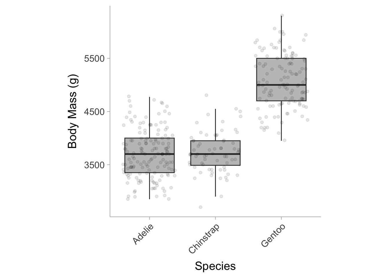
By default, summary.aov() does not report the \(\eta^2\) value (i.e., the variance explained by species), however we will discuss this more in Section 10.7.1. The results show that the mean body mass between the three penguin species (Adelie, Gentoo, Chinstrap) differ significantly from one another (see Figure 10.1).

Figure 10.1: Box plots showing the distribution of body mass by species.

10.3 One-way between-subjects ANOVA

One-way between-subject ANOVA is an extension of independent-samples t-tests. The null hypothesis is that all k means of k independent groups are identical, whereas the alternative hypothesis is that there are at least one mean that differs from the other groups. The assumptions include: (1) independence of observations, (2) normality of residuals, and (3) equality (or homogeneity) of variances (homoscedasticity).¹

Note, sometimes you may encounter a between-subject one-way ANOVA which compares only two conditions, particularly when the paper is old. This is essentially a t-test, and the F-statistic is just \(\mathsf{t^2}\). It is preferable to report Cohen’s d as a effect size in two group comparisons as opposed to \(\eta^2\) and, fortunately, we can convert \(\eta^2\) to a Cohen’s d. It is recommended that subsequent analyses (e.g., power analysis) of two group comparisons are based on Cohen’s d.

10.3.1 Determining degrees of freedom for one-way ANOVAs

Please refer to the following table to determine the degrees of freedom for ANOVA effects, if they are not reported or if you suspect that they have been misreported.

Degrees of freedom
Between subjects ANOVA
Effect	\(k-1\)
Error	\(n-k\)
Total	\(n-1\)

10.3.2 Calculating eta-squared from F-statistic and degrees of freedom

Using the formula below, we can calculate \(\eta^2\) of an ANOVA model using the F-statistic and the degrees of freedom,

\[ \eta^2 = \frac{df_\text{effect}\times F}{df_\text{effect} \times F + df_\text{error}}. \]

Where \(df_\text{error}\) and \(df_\text{effect}\) denotes the degrees of freedom for the residual error term and the main effect, respectively. In R, we can use the F_to_eta2() function from the effectsize package (Ben-Shachar, Lüdecke, and Makowski 2020):

library(effectsize)

n = 154 # number of subjects
k = 3 # number of groups
f = 84.3 # F-statistic

# get degrees of freedom
df_effect = k - 1
df_error = n - k

# calculate eta-squared
F_to_eta2(f = f,
          df = df_effect,
          df_error = df_error,
          alternative = 'two.sided') # obtain two sided CIs

Eta2 (partial) |       95% CI
-----------------------------
0.53           | [0.42, 0.61]

The results of this example show an \(\eta^2\) value of .53 95% CI [.42, .61]. This suggests that the grouping variable accounts for 53% of the total variation in the outcome.

10.3.3 Calculating eta-squared from an ANOVA table

Let’s use the table from the ANOVA model in Section 10.2 that pertains to the effect of penguin species on body mass:

One-way ANOVA table

	Df	Sum Sq	Mean Sq	F value	Pr(>F)
species	2	146864214	73432107.1	343.6263	0
Residuals	339	72443483	213697.6	NA	NA

From this table we can use the sum of squares from the grouping variable (species) and the total sum of squares (\(SS_\text{total} = SS_\text{effect} + SS_\text{error}\)) to calculate the \(\eta^2\) value using the following equation:

\[ \eta^2 = \frac{SS_\text{effect}}{SS_\text{total}} = \frac{SS_\text{effect}}{SS_\text{effect} + SS_\text{error}} \]

In R, we can use the eta.full.SS() or eta.F() function in the MOTE package (Buchanan et al. 2019) to obtain \(\eta^2\) from an ANOVA table.

library(MOTE)

# calculate eta-squared with eta.full.SS
eta <- eta.full.SS(dfm = 2,  # effect degrees of freedom
                   dfe = 339, # error degrees of freedom
                   ssm = 146864214, # sum of squares for the effect
                   sst = 146864214 + 72443483, # total sum of squares
                   Fvalue = 343.6263,
                   a = .05)

# display results
data.frame(eta_squared = round(eta$eta,3),
           ci.lb = round(eta$etalow,3),
           ci.ub = round(eta$etahigh,3))

  eta_squared ci.lb ci.ub
1        0.67 0.606 0.722

# alternative approach with eta.F
eta <- eta.F(dfm = 2,  # effect degrees of freedom
             dfe = 339, # error degrees of freedom
             Fvalue = 343.6263,
             a = .05)

# display results
data.frame(eta_squared = round(eta$eta,3),
           ci.lb = round(eta$etalow,3),
           ci.ub = round(eta$etahigh,3))

  eta_squared ci.lb ci.ub
1        0.67 0.606 0.722

The example code outputs \(\eta^2\) = .67 [.61, .72]. This suggests that species accounts for 67% of the total variation in body mass between penguins.

10.3.4 Calculating Cohen’s d for post-hoc comparisons

In an omnibus ANOVA, the p-value is telling us whether the means from all groups come from the same population mean, however this does not inform us about which group means differ or by how much. Using the same example as before, let’s say we want to answer a specific question such as: what is the difference in body mass between Adelie penguins and Gentoo penguins? To answer this question, we can calculate the raw mean difference between the two groups. In R, we can do that with the following code:

library(tidyverse)

# get means for each species
stats <- penguins %>%
  summarize(mean = mean(body_mass_g, na.rm = TRUE), 
            .by = species)

# display means
stats

# A tibble: 3 × 2
  species    mean
  <fct>     <dbl>
1 Adelie    3701.
2 Gentoo    5076.
3 Chinstrap 3733.

# get raw mean difference
stats$mean[2] - stats$mean[1]

[1] 1375.354

Based on the mean difference, Gentoo penguins are on average 1375 grams heavier than Adelie penguins in total body mass. We can also calculate a standardized mean difference using the escalc() function in the metafor package (Viechtbauer 2010).

library(metafor)

# Means, SDs, and sample sizes for each species
stats <- penguins %>%
  summarize(mean = mean(body_mass_g, na.rm = TRUE), 
            sd = sd(body_mass_g, na.rm = TRUE), 
            n = n(),
            .by = species)

# show table of stats
stats

# A tibble: 3 × 4
  species    mean    sd     n
  <fct>     <dbl> <dbl> <int>
1 Adelie    3701.  459.   152
2 Gentoo    5076.  504.   124
3 Chinstrap 3733.  384.    68

# calculate standardized mean difference
effect_size <- escalc(measure = 'SMD',
                      m1i = stats$mean[2],
                      m2i = stats$mean[1],
                      sd1i = stats$sd[2],
                      sd2i = stats$sd[1],
                      n1i = stats$n[2],
                      n2i = stats$n[1],
                      var.names = c("d","variance"))

# display results
summary(effect_size)

       d variance    sei      zi   pval  ci.lb  ci.ub 
1 2.8602   0.0295 0.1716 16.6629 <.0001 2.5237 3.1966 

The standardized mean difference between Adelie and Gentoo penguins is \(d\) = 2.86 95% CI [2.52, 3.19], demonstrating that Gentoo penguins have body mass 2.86 standard deviations larger than Adelie penguins.

We can also quantify contrasts from summary statistics reported from the ANOVA table and the group means (labeled group \(A\) and \(B\)). We can calculate the standardized mean difference using the means from both groups and the mean squared error (\(MSE\); i.e., the mean square of the residuals) the following equation:

\[ d = \frac{M_A - M_B}{\sqrt{MSE}} \]

This method gives a standardized mean difference equivalent to the Cohen’s \(d\) with the pooled standard deviation in the denominator (see chapter on mean differences). Therefore if we obtain the mean squared errors from Section 10.3.3 and we obtain the means (means: Gentoo = 5076, Adelie = 3701), we can calculate the standardized mean difference as: \(\frac{5076 - 3701}{\sqrt{213697.6}} = \frac{1375}{462.27 } = 2.974\). The discrepency between the standardized mean difference provided by the escalc() function is due to the fact that the function automatically applies a small sample correction factor (i.e., Hedges’ g) thus reducing the overall effect (see the small sample bias section in the mean differences chapter).

	Df	Sum Sq	Mean Sq	F value	Pr(>F)
species	2	146864214	73432107.1	343.6263	0
Residuals	339	72443483	213697.6	NA	NA

Beware the assumptions.

Note that this method is ONLY valid when you are willing to assume equal variances among groups (homoscedasticity), and when you conduct a Fisher’s one-way ANOVA (rather than Welch’s). This method is also impractical if you are calculating from reported statistics, and MSE is not reported (which is typically the case).

If you are unwilling to assume homogeneity of variances, you should know it also that it also makes little sense to conduct a Fisher’s ANOVA in such situations. You may want to switch to Welch’s ANOVA, which does not assume homoscedasticity. For comparisons between groups with unequal variances you may want to use an alternative standardized effect size measure, such as Glass’ delta.

10.4 One-way repeated measures ANOVA

One-way repeated measures ANOVA (rmANOVA) is an extension of paired-samples t-tests, with the difference being it can be used in two or more groups.

10.4.1 Determining degrees of freedom for one-way rmANOVA

Please refer to the following table to determine the degrees of freedom for repeated measure ANOVA effects.

Degrees of freedom
Within-subject ANOVA (repeated measures)
Effect	\(k-1\)
Error-between	\((n-1)\times(k-1)\)
Error-within	\((n-1)\cdot (k-1)\)
Total (within)	\(n\cdot (k-1)\)

10.4.2 Eta-squared from rmANOVA statistics

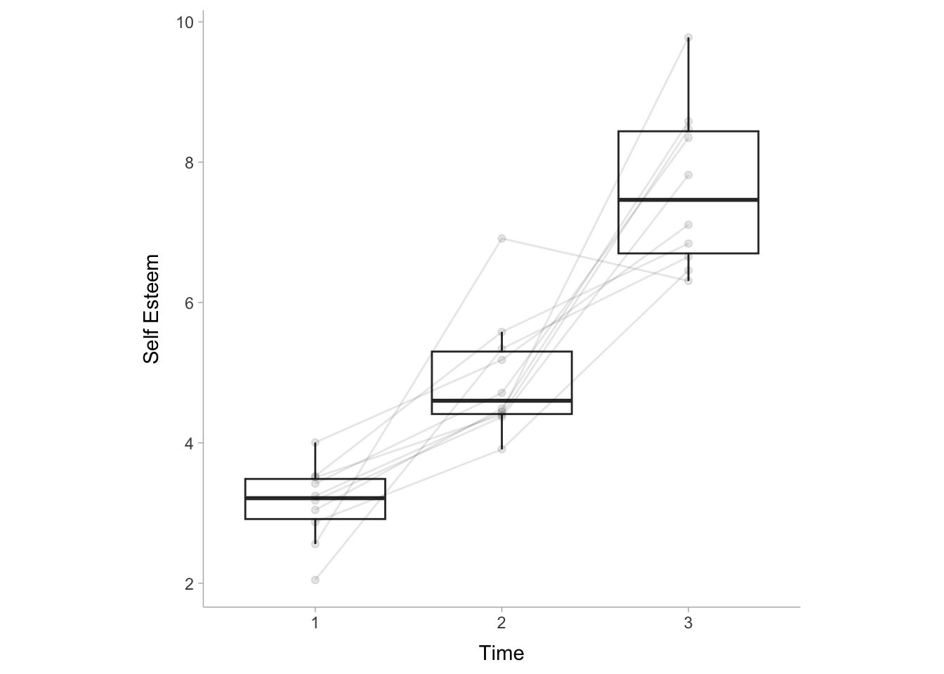
Commonly, we use eta-squared (\(\eta^2\)) or partial eta-squared (\(\eta_p^2\)) as the effect size measure for one-way rmANOVAs, for which these two are in fact equal. Let’s construct an rmANOVA model using example data from the datarium package (Kassambara 2019). The selfesteem data set simply shows self-esteem scores over three repeated measurements within the same subjects (see Figure 10.2).

Figure 10.2: Box plot of self esteem at each time point. Lines connect subjects across time points.

Let’s get the ANOVA results in R,

# load in data 
data("selfesteem", package = "datarium")

# reformat data
selfesteem <- selfesteem %>%
  pivot_longer(cols = c("t1","t2","t3"),
               names_to = "time",
               values_to = "self_esteem") %>%
  rename(subject = id)

# display data
head(selfesteem)

# A tibble: 6 × 3
  subject time  self_esteem
    <int> <chr>       <dbl>
1       1 t1           4.01
2       1 t2           5.18
3       1 t3           7.11
4       2 t1           2.56
5       2 t2           6.91
6       2 t3           6.31

# fit ANOVA
rmANOVA_mdl = aov(formula = self_esteem ~ time + Error(subject),
                  data = selfesteem)

# display ANOVA table
summary(rmANOVA_mdl)

Error: subject
          Df  Sum Sq Mean Sq F value Pr(>F)
Residuals  1 0.07667 0.07667               

Error: Within
          Df Sum Sq Mean Sq F value   Pr(>F)    
time       2 102.46   51.23   63.07 1.06e-10 ***
Residuals 26  21.12    0.81                     
---
Signif. codes:  0 '***' 0.001 '**' 0.01 '*' 0.05 '.' 0.1 ' ' 1

There are two tables displayed here, the table on top displays the between subject effects and the table below shows the within subject effects. The equations and functions to calculate \(\eta^2\) mentioned in the one-way between-subjects ANOVAs section also apply here:

\[ \eta^2 = \frac{df_\text{effect}\times F}{df_\text{effect} \times F + df_\text{error-within}}, \]

\[ \eta^2 = \frac{SS_\text{effect}}{SS_\text{total}}. \]

Note that here \(SS_\text{total}\) does not include \(SS_\text{error-between}\) because we are not interested in the between-subject variance since we are conducting a rmANOVA. In other words, between-subjects variance can be large or small, but we do not care about it when we examine whether there is an effect within subjects. Therefore the total sum of squares can be defined as

\[ SS_\text{total} = SS_\text{effect} + SS_\text{error-within}. \]

As a result, we can calculate \(\eta^2\) from the rmANOVA table as,

\[ \eta^2 = \frac{102.46}{21.12 + 102.46} = .83 \]

We can plug the rmANOVA model into the eta_squared() function from the effectsize package in R (Ben-Shachar, Lüdecke, and Makowski 2020) to calculate \(\eta^2\).

library(effectsize)

# calculate eta-squared
eta_squared(rmANOVA_mdl,
            alternative = "two.sided")

# Effect Size for ANOVA (Type I)

Group  | Parameter | Eta2 (partial) |       95% CI
--------------------------------------------------
Within |      time |           0.83 | [0.69, 0.89]

As expected, we find the same point-estimate from our hand calculation. To calculate \(\eta^2\) from the F-statistic and degrees of freedom we can use the MOTE package (Buchanan et al. 2019) as we did in Section 10.3.3:

library(MOTE)

# calculate eta squared
eta <- eta.full.SS(dfm = 2,  # effect degrees of freedom
                   dfe = 26, # error degrees of freedom
                   ssm = 102.46, # sum of squares for the effect
                   sst = 102.46 + 21.12, # total sum of squares
                   Fvalue = 63.07,
                   a = .05)

# display results
data.frame(eta_squared = round(eta$eta,3),
           ci.lb = round(eta$etalow,3),
           ci.ub = round(eta$etahigh,3))

  eta_squared ci.lb ci.ub
1       0.829 0.644  0.91

The results show \(\eta^2\) = .83 95% CI [.64, .91]. Note there is a slight discrepancy in the calculation of confidence intervals between the MOTE and effectsize package.

10.5 Two-way between-subjects ANOVA

Two-way between-subjects ANOVA is used when there are two predictor grouping variables in the model. Note again that “between-subjects” means that each group contains different subjects.

10.5.1 Determining degrees of freedom

Please refer to the following table to determine the degrees of freedom for two-way ANOVA effects (Morse 2018). Note that \(k_1\) is the number of groups in the first variable, and \(k_2\) is the number of groups in the second variable.

Degrees of freedom
Within subjects ANOVA
Main Effect (of one variable)	\(k_1-1\) or \(k_2-1\)
Interaction Effect	\((k_1-1)\times (k_2-1)\)
Error	\(n-k_1\cdot k_2\)
Total	\(n-1\)

10.5.2 Eta-squared from two-way ANOVA statistics

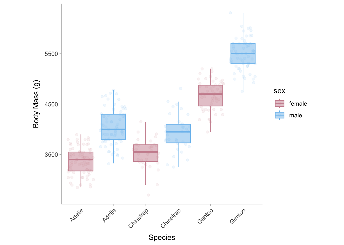
For two-way ANOVAs we can obtain the partial eta-squared \((\eta^2_p)\) for each predictor in the model. Let’s construct our ANOVA model using data from the palmerpenguins dataset (Horst, Hill, and Gorman 2020). In this example we want to see how the species and the sex of the penguin explains variance in body mass (see Figure 10.3).

Figure 10.3: Box plots of body mass for each penguin species and sex.

Let’s load in the data set and fit the two-way ANOVA model and display the table.

library(palmerpenguins)

ANOVA2_mdl <- aov(body_mass_g ~ species + sex + species:sex,
                  data = penguins)

summary(ANOVA2_mdl)

             Df    Sum Sq  Mean Sq F value   Pr(>F)    
species       2 145190219 72595110 758.358  < 2e-16 ***
sex           1  37090262 37090262 387.460  < 2e-16 ***
species:sex   2   1676557   838278   8.757 0.000197 ***
Residuals   327  31302628    95727                     
---
Signif. codes:  0 '***' 0.001 '**' 0.01 '*' 0.05 '.' 0.1 ' ' 1
11 observations deleted due to missingness

The results show that species, sex, and the interaction between the two account for substantial variance in body mass. We can obtain the contributions of species, sex, and their interaction by computing the partial eta-squared value (\(\eta_p^2\)) for each. To do this, we can use similar formulas to \(\eta^2\) from the one-way ANOVA. The difference between the formulas for \(\eta_p^2\) and \(\eta^2\) is that \(\eta_p^2\) does not use the total sum of squares in the denominator, instead it uses the residual sum of squares (\(SS_\text{error}\)) and the sum of squares from the effect of interest (\(SS_\text{effect}\)). For example,

\[ \text{For species:}\;\;\;\; \eta_p^2= \frac{SS_\text{effect}}{SS_\text{effect} + SS_\text{error}} = \frac{145190219}{145190219+ 31302628} = .82 \] \[ \text{For sex:}\;\;\;\; \eta_p^2= \frac{SS_\text{effect}}{SS_\text{effect} + SS_\text{error}} = \frac{37090262}{37090262 + 31302628} = .54 \] \[ \text{For sex}\times\text{species:}\;\;\;\; \eta_p^2= \frac{SS_\text{effect}}{SS_\text{effect} + SS_\text{error}} = \frac{1676557}{1676557+ 31302628} = .05 \] We can also easily do this in R using the eta_squared function in the effectsize package (Ben-Shachar, Lüdecke, and Makowski 2020) and setting the argument partial = TRUE.

# calculate partial eta-squared
eta_squared(ANOVA2_mdl,
            partial = TRUE,
            alternative = "two.sided")

# Effect Size for ANOVA (Type I)

Parameter   | Eta2 (partial) |       95% CI
-------------------------------------------
species     |           0.82 | [0.79, 0.85]
sex         |           0.54 | [0.48, 0.60]
species:sex |           0.05 | [0.01, 0.10]

The results show the \(\eta_p^2\) value and 95% CIs for each term in the ANOVA model.

10.6 Two-way repeated measures ANOVA

A two-way repeated measures ANOVA (rmANOVA) would indicate that subjects are exposed to each condition along two variables.

10.6.1 Determing degrees of freedom

Please refer to the following table to determine the degrees of freedom for two-way rmANOVA effects (Morse 2018). Note that \(k_1\) is the number of groups in the first variable, and \(k_2\) is the number of groups in the second variable.

Degrees of freedom
Between subjects ANOVA
Main Effect (of one variable)	\(k_1-1\) or \(k_2-1\)
Interaction Effect	\((k_1-1)\times (k_2-1)\)
Error-between	\((k_1 \cdot k_2) - 1\)
Error-within	\((n - 1)\times (k_1\cdot k_2 - 1)\)
Total	\(n-1\)

10.6.2 Eta-squared from Two-way rmANOVA

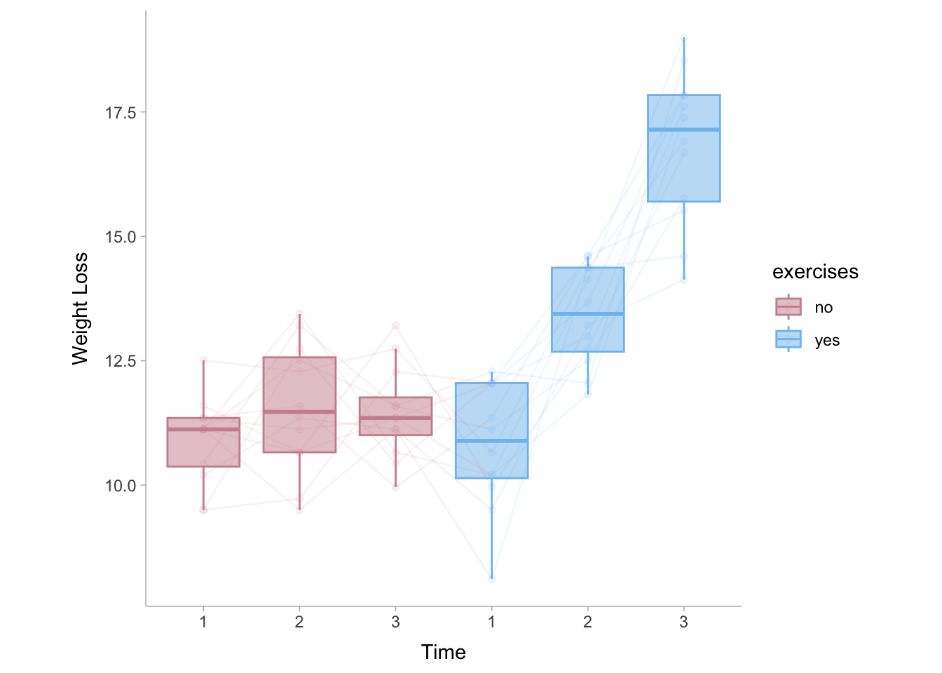
For a two-way repeated measures ANOVA, we can use the weightloss data set from the datarius package (Kassambara 2019). This data set contains a diet condition and a control condition that tracked subjects across time (3 time points) for each of condition (see Figure 10.4).

Figure 10.4: Box plots showing the weight loss across time points and conditions. Lines connect subjects across conditions.

Let’s conduct a two-way rmANOVA in R.

### load in data
data("weightloss", package = "datarium")

# reformat data
weightloss <- weightloss  %>% 
  pivot_longer(cols = c("t1","t2","t3"),
               names_to = "time",
               values_to = "weight_loss") %>%
  rename(subject = id) %>%
  filter(diet=='no')

# fit ANOVA model
rmANOVA2_mdl = aov(formula = weight_loss ~ time + exercises + time:exercises + Error(subject),
                   data = weightloss)

# display ANOVA table
summary(rmANOVA2_mdl)

Error: subject
          Df Sum Sq Mean Sq F value Pr(>F)
Residuals 11  20.64   1.877               

Error: Within
               Df Sum Sq Mean Sq F value   Pr(>F)    
time            2 129.26   64.63   50.57 3.45e-13 ***
exercises       1 101.03  101.03   79.05 3.16e-12 ***
time:exercises  2  92.55   46.28   36.21 9.26e-11 ***
Residuals      55  70.29    1.28                     
---
Signif. codes:  0 '***' 0.001 '**' 0.01 '*' 0.05 '.' 0.1 ' ' 1

From the table and graph above, we can see that there is substantial within-person change in weight loss under the exercise condition and no discernible increase in weight loss without exercising. This suggests that there is a substantial interaction effect. Like we did in the between-subjects two-way ANOVA, we can calculate the partial eta squared values from the ANOVA table

\[ \text{For time:}\;\;\;\; \eta_p^2= \frac{SS_\text{effect}}{SS_\text{effect} + SS_\text{error-within}} = \frac{129.26}{129.26+ 70.29} = .65 \] \[ \text{For exercise:}\;\;\;\; \eta_p^2= \frac{SS_\text{effect}}{SS_\text{effect} + SS_\text{error-within}} = \frac{101.03}{101.03 + 70.29} = .59 \] \[ \text{For sex}\times\text{species:}\;\;\;\; \eta_p^2= \frac{SS_\text{effect}}{SS_\text{effect} + SS_\text{error-within}} = \frac{92.55}{92.55+ 70.29} = .57 \]

Remember for the partial eta-squared, the denominator is not the total sum of squares rather it is the effect sum of squares and the error. In the repeated measures ANOVA, the error should only be for the within subject error because the variance between subjects is not something we are interested in. We can also calculate this in R using the eta_squared() function again.

# calculate partial eta-squared
eta_squared(rmANOVA2_mdl,
            partial = TRUE,
            alternative = "two.sided")

# Effect Size for ANOVA (Type I)

Group  |      Parameter | Eta2 (partial) |       95% CI
-------------------------------------------------------
Within |           time |           0.65 | [0.49, 0.75]
Within |      exercises |           0.59 | [0.42, 0.70]
Within | time:exercises |           0.57 | [0.39, 0.69]

The results show the \(\eta_p^2\) value and 95% CIs for each term in the rmANOVA model.

10.7 Effect Sizes for ANOVAs

ANOVA (Analysis of Variance) is a statistical method used to compare means across multiple groups or conditions. It is mostly used when the outcome variable is continuous and the predictor variables are categorical. Commonly used effect size measures for ANOVAs / F-tests include: eta-squared (\(\eta^2\)), partial eta-squared (\(\eta_p^2\)), generalized eta-squared (\(\eta^2_G\)), omega-squared (\(\omega^2\)), partial omega-squared (\(\omega\)), generalized omega-squared (\(\omega^2_G\)), Cohen’s \(f\).

Type	Description	Section
\(\eta^2\) - eta-squared	Measures the variance explained of the whole ANOVA model.	Section 10.7.1
\(\eta^2_p\) - Partial eta-squared	Measures the variance explained by a specific factor in the model.	Section 10.7.2
\(\eta^2_G\) - Generalized eta-squared	Similar to \(\eta^2\), but uses the sum of squares of all non-manipulated variables in the calculation. This allows meta-analysts to compare \(\eta_G\) across different designs.	Section 10.7.3
\(\omega^2,\omega^2_p,\omega^2_G\) - Omega squared corrections	Corrections to bias observed in \(\eta^2\) measures. Can be interpreted in the same way as \(\eta^2\).	Section 10.7.4
\(f\) - Cohen’s f	This effect size can be interpreted as the average Cohen’s \(d\) between each group.	Section 10.7.5

10.7.1 Eta-Squared (\(\eta^2\))

Eta-squared is the ratio between the between-group variance and the total variance. It describes the proportion of the total variability in the data that are accounted for by a factor. Therefore, it is a measure of variance explained. To calculate eta-squared (\(\eta^2\)) we need to first calculate the total sum of squares (\(SS_{\text{total}}\)) and the effect sum of squares (\(SS_{\text{effect}}\)),

\[ SS_{\text{total}} = \sum_{i=1}^n (y_i-\bar{y})^2 \tag{10.1}\]

Where \(\bar{y}\) is the grand mean (i.e., the mean of all data points collapsed across groups) and \(y_i\) is the outcome value for observation \(i\). To calculate the sum of squares of the effect, we can use predicted outcome values (\(\hat{y}_i\)) rather than the raw outcome values (\(y_i\)). In the case of categorical predictors, \(\hat{y}_i\) is equal to the mean of the outcome within that individual’s respective group. Therefore the sum of squares of the effect can be calculated using the following formula:

\[ SS_{\text{effect}} = \sum_{i=1}^n (\hat{y}_i-\bar{y})^2. \tag{10.2}\]

Now we can calculate the \(\eta^2\) value,

\[ \eta^2 = \frac{SS_{\text{effect}}}{SS_{\text{total}}} \tag{10.3}\]

The standard error of \(\eta^2\) can be approximated from Olkin and Finn (1995):

\[ SE_{\eta^2}=\sqrt{\frac{4\eta^2\left(1-\eta^2\right)^2\left(n+k-1\right)^2}{\left(n^2-1\right)\left(3+n\right)}} \tag{10.4}\]

The sampling distribution for \(\eta^2\) is asymmetric as all the values are bounded in the range, 0 to 1. The confidence interval surrounding \(\eta^2\) will likewise be asymmetric so instead of calculating the confidence interval from the standard error, we can instead use a non-central F-distribution using the degrees of freedom between groups (e.g., for three groups: \(df_b=k-1=3-1=2\)) and the degrees of freedom within groups (e.g., for 100 subjects and three groups: \(df_b=n-k=100-3=97\)) to obtain the confidence intervals (this is done automatically in the effectsize package). Another option is to use bootstrapping procedure (i.e., resampling the observed data points to construct a sampling distribution around \(\eta^2\), see Kirby and Gerlanc 2013) and then take the .025 and .975 quantiles of that distribution.

In R, we can calculate \(\eta^2\) from a one-way ANOVA using the palmerpenguins data set. The aov function in base R allows the analyst to model an ANOVA with categorical predictors on the right side (species) of the ~ and the outcome on the left side (body mass of penguin). We can then use the eta_squared function in the effectsize package to calculate the point estimate and confidence intervals.

# Example:
# group: species
# outcome: body mass

# One-Way ANOVA
mdl1 <- aov(data = penguins,
           body_mass_g ~ species)

# calculate eta-squared
eta_squared(mdl1, 
            partial = FALSE,
            alternative = "two.sided")

# Effect Size for ANOVA (Type I)

Parameter | Eta2 |       95% CI
-------------------------------
species   | 0.67 | [0.62, 0.71]

The species of the penguin explains the majority of the variation in body mass showing an eta-squared value of \(\eta^2\) = .67 [.62, .71]. Let us now do the same thing with a two-way ANOVA, using both species and sex as our categorical predictors.

# Example:
# group: species and sex
# outcome: body mass

# Two-Way ANOVA
mdl2 <- aov(data = penguins,
            body_mass_g ~ species + sex)

# calculate eta-squared
eta_squared(mdl2, 
            partial = FALSE,
            alternative = "two.sided")

# Effect Size for ANOVA (Type I)

Parameter | Eta2 |       95% CI
-------------------------------
species   | 0.67 | [0.62, 0.72]
sex       | 0.17 | [0.10, 0.24]

Notice that the \(\eta^2\) does not change for species since the sum of squares is divided by the total sum of squares rather than the residual sum of squares (see partial eta squared). The example shows an eta-squared value for species of \(\eta^2\) = .67 95% CI [.62, .72] and for sex \(\eta^2\) = .17 95% CI [.10, .24].

10.7.2 Partial Eta-Squared (\(\eta^2_p\))

Partial eta-squared is the most commonly reported effect size measure for F-tests. It describes the proportion of variability associated with an effect when the variability associated with all other effects identified in the analysis has been removed from consideration (hence, it is “partial”). If you have access to an ANOVA table, the partial eta-squared for an effect is calculated as:

\[ \eta_p^2 = \frac{ SS_{\text{effect}}}{SS_{\text{effect}}+SS_{\text{error}}} \tag{10.5}\]

There are two things to take note of here:

1. In a one-way ANOVA (one categorical predictor), partial eta-squared and eta-squared are equivalent since \(SS_{\text{total}} = SS_{\text{effect}}+SS_{\text{error}}\)
2. If there are multiple predictors, the denominator will only include the sum of squares of the effect of interest (+ residuals) rather than the effect of all predictors (which is the case for the non-partial eta squared).

In R, let us compare the partial eta-squared values for a one-way ANOVA and a two-way ANOVA using the eta_squared function in the effectsize package.

# Example:
# group: species
# outcome: body mass


# one-way ANOVA
mdl1 <- aov(data = penguins,
           body_mass_g ~ species)

# calculate eta-square
eta_squared(mdl1, 
            partial = TRUE,
            alternative = "two.sided") 

For one-way between subjects designs, partial eta squared is equivalent
  to eta squared. Returning eta squared.

# Effect Size for ANOVA

Parameter | Eta2 |       95% CI
-------------------------------
species   | 0.67 | [0.62, 0.71]

The species of the penguin explains the majority of the variation in body mass showing a partial eta-squared value of \(\eta^2\) = \(\eta^2_p\) = .67 95% CI [.62, .71]. Let us now do the same thing with a two-way ANOVA, using both species and sex as our categorical predictors.

# Example:
# group: species and sex
# outcome: body mass

# two-way ANOVA
mdl2 <- aov(data = penguins,
           body_mass_g ~ species + sex)

# calculate eta-squared
eta_squared(mdl2, 
            partial = TRUE,
            alternative = "two.sided")

# Effect Size for ANOVA (Type I)

Parameter | Eta2 (partial) |       95% CI
-----------------------------------------
species   |           0.81 | [0.78, 0.84]
sex       |           0.53 | [0.46, 0.59]

Once we run a two-way ANOVA, the partial eta-squared value for species begins to differ. The example shows a partial eta-squared value for species of \(\eta^2_p\) = .81 95% CI [.78, .84] and for sex \(\eta^2\) = .53 95% CI [.46, .59].

10.7.3 Generalized Eta-Squared (\(\eta^2_G\))

Generalized eta-squared was devised to allow effect size comparisons across studies with different designs, which eta-squared and partial eta-squared cannot help with (refer to for details). If you can (either you are confident that you calculated it right, or the statistical software that you use just happens to return this measure), report generalized eta-squared in addition to eta-squared or partial eta-squared. The biggest advantage of generalized eta-squared is that it facilitates meta-analysis, which is important for the accumulation of knowledge. To calculate generalized eta-squared, the denominator should be the sums of squares of all the non-manipulated variables (i.e., variance of purely individual differences in the outcome rather than individual differences in treatment effects). Note the formula will depend on the design of the study. In R, the eta_squared function in the effectsize package supports the calculation of generalized eta-squared by using the generalized=TRUE argument.

10.7.4 Omega squared corrections (\(\omega^2\), \(\omega^2_p\))

Similar to Hedges’ correction for small sample bias in standardized mean differences, \(\eta^2\) is also biased. We can apply a correction to \(\eta^2\) and obtain a relatively unbiased estimate of the population proportion of variance explained by the predictor. To calculate \(\omega\), we need to calculate the within group mean squared errors:

\[ MSE_{\text{within}} = \frac{1}{n}\sum_{i=1}^n (y_i-\hat{y}_i)^2. \] Where the predicted values of the outcome, \(\hat{y}_i\), are the mean value for the individual’s respective group. The formula for \(\omega^2\) is,

\[ \omega^2 = \frac{SS_{\text{effect}}-(k-1)\times MSE_{\text{within}}}{SS_{\text{total}} + MSE_{\text{within}}} \tag{10.6}\]

Where \(k\) is the number of groups in the predictor (effect) variable. For partial omega-squared values, we need the mean squared error of the effect and the residuals which can easily be calculated from their sum of squares:

\[ MSE_{\text{effect}} = \frac{SS_{\text{effect}}}{n} \tag{10.7}\]

\[ MSE_\text{error} = \frac{SS_{\text{error}}}{n} \tag{10.8}\]

Then to calculate the partial omega squared we can use the following formula:

\[ \omega_p^2 = \frac{(k-1)(MSE_{\text{effect}} - MSE_{\text{error}})}{(k-1)\times MSE_{\text{effect}} + (n-k-1)\times MSE_{\text{error}}} \tag{10.9}\]

In R, we can use the omega_squared function in the effectsize package to calculate both \(\omega^2\) and \(\omega^2_p\). For the first example we will use a one-way ANOVA.

# Example:
# group: species
# outcome: body mass

# One-Way ANOVA
mdl1 <- aov(data = penguins,
           body_mass_g ~ species)

# omega-squared
omega_squared(mdl1, 
              partial = FALSE,
              alternative = "two.sided")

# Effect Size for ANOVA (Type I)

Parameter | Omega2 |       95% CI
---------------------------------
species   |   0.67 | [0.61, 0.71]

# partial omega-squared
omega_squared(mdl1, 
              partial = TRUE,
              alternative = "two.sided")

For one-way between subjects designs, partial omega squared is
  equivalent to omega squared. Returning omega squared.

# Effect Size for ANOVA

Parameter | Omega2 |       95% CI
---------------------------------
species   |   0.67 | [0.61, 0.71]

The species of the penguin explains the majority of the variation in body mass, showing an omega-squared value of \(\omega^2\) = .67 95% CI [.61, .71]. Note that the partial and non-partial omega squared values do not show a difference as expected in a one-way ANOVA. Let us now do the same thing with a two-way ANOVA, using both species and sex as our categorical predictors.

# Example:
# group: species and sex
# outcome: body mass

# Two-Way ANOVA
mdl2 <- aov(data = penguins,
           body_mass_g ~ species + sex)

# omega-squared
omega_squared(mdl2, 
            partial = FALSE,
            alternative = "two.sided")

# Effect Size for ANOVA (Type I)

Parameter | Omega2 |       95% CI
---------------------------------
species   |   0.67 | [0.62, 0.72]
sex       |   0.17 | [0.10, 0.24]

# partial omega-squared
omega_squared(mdl2, 
              partial = TRUE,
              alternative = "two.sided")

# Effect Size for ANOVA (Type I)

Parameter | Omega2 (partial) |       95% CI
-------------------------------------------
species   |             0.81 | [0.78, 0.84]
sex       |             0.53 | [0.46, 0.58]

Once we run a two-way ANOVA, the partial eta-squared value for species diverge. The example shows a partial eta-squared value for species of \(\omega^2_p\) = .81 95% CI[.78, .84] and for sex \(\omega^2\) = .53 95% CI [.46, .58].

10.7.5 Cohen’s \(f\)

Cohen’s \(f\) is defined as the ratio of the between-group standard deviation to the within-group standard deviation (note that ANOVA assumes equal variances among groups). Cohen’s \(f\) is the effect size measure asked for by G*Power for power analysis for F-tests. This can be calculated easily from the eta-squared value,

\[ f = \sqrt{\frac{\eta^2}{1-\eta^2}} \tag{10.10}\]

or by the \(\omega^2\) value,

\[ f = \sqrt{\frac{\omega^2}{1-\omega^2}} \tag{10.11}\]

Cohen’s \(f\) can be interpreted as “the average Cohen’s \(d\) (i.e., standardized mean difference) between groups”. Note that there is no directionality to this effect size (\(f\) is always greater than zero), therefore two studies showing the same \(f\) with the same groups, can have very different patterns of group mean differences. Also note that Cohen’s \(f\) is often reported as \(f^2\). The confidence intervals for Cohen’s \(f\) can be computed from the upper bounds and lower bounds of the confidence intervals from eta-square or omega-square using the formulas to calculate \(f\) (e.g., for the upper bound \(f_{UB} = \sqrt{\frac{\eta^2_{UB}}{1-\eta^2_{UB}}}\)).

In R, we can use the cohens_f() function in the effectsize package to calculate Cohen’s \(f\). We can also get \(f\) from \(eta^2\) value using the eta2_to_f() function. We will again use example data from the palmerpenguins package.

# Example:
# group: species
# outcome: body mass

# fit ANOVA model
mdl <- aov(data = penguins,
           body_mass_g ~ species)   

# calculate Cohen's f from anova table
cohens_f(mdl,alternative = "two.sided")

For one-way between subjects designs, partial eta squared is equivalent
  to eta squared. Returning eta squared.

# Effect Size for ANOVA

Parameter | Cohen's f |       95% CI
------------------------------------
species   |      1.42 | [1.27, 1.57]

# code for calculating f from eta2
# get eta squared values
eta_values <- eta_squared(mdl,alternative = "two.sided")

For one-way between subjects designs, partial eta squared is equivalent
  to eta squared. Returning eta squared.

# calculate f from eta
data.frame(f = eta2_to_f(eta_values$Eta2),
           ci.lb = eta2_to_f(eta_values$CI_low),
           ci.ub = eta2_to_f(eta_values$CI_high))

         f    ci.lb    ci.ub
1 1.423831 1.271129 1.573348

In the example above, the difference in body mass between the three penguin species was very large showing a Cohen’s \(f\) of 1.42 95% CI [1.27, 1.57].

10.8 Reporting ANOVA results

For ANOVAs/F-tests, you will always need to report two kinds of effects: the omnibus effect of the factor(s) and the effect of planned contrasts or post hoc comparisons.

For instance, imagine that you are comparing three groups/conditions with a one-way ANOVA. The ANOVA will first return an F-statistic, the degrees of freedom, and the associated p-value. Here, you need to calculate the size of this omnibus factor effect in eta-squared, partial eta-squared, or generalized eta-squared. Suppose the omnibus effect is significant. You now know that there is at least one group that differs from the others. You want to know which group(s) differ from the others, and how much they differ. Therefore, you conduct post hoc comparisons on these groups. Because post hoc comparisons compare each group with the others in pairs, you will get a t-statistic and p-value for each comparison. For this, you need to calculate and report the standardized mean difference (\(d\)).

Imagine instead that you have two independent variables or factors, and you conduct a two-by-two factorial ANOVA. The first thing to do then is look at the interaction. If the interaction is significant, you again report the associated omnibus effect size measures, and proceed to analyze the simple effects. Depending on your research question, you compare the levels of one independent variable on each level of the other independent variable. You will report \(d\) for these simple effects. If the interaction is not significant, you look at the main effects and report the associated omnibus effect. You then proceed to analyze the main effect by comparing the levels of one independent variable while collapsing/aggregating the levels of the other independent variable. You will report \(d\) for these pairwise comparisons.

Note that lower-order effects are not directly interpretable if you have higher order effects. If you have an interaction in a two-way ANOVA, you cannot interpret the main effects directly. If you have a three-way interaction in a three-way ANOVA, you cannot interpret the main effects or the two-way interactions directly, regardless of whether they are significant or not.

In R, we can use the summary function to display the anova table. We can also append the table to include, for example, partial omega squared values and their respective confidence intervals.

# ANOVA mdl
mdl <- aov(data = penguins,
           body_mass_g ~ species + sex)   

# calculate partial omega-squared values
omega_values <- omega_squared(mdl, alternative = "two.sided")

# create table of partial omega-squared values
omega_table <- data.frame(omega_sq = round(c(omega_values$Omega2_partial,NA),3),
                     ci.lb = round(c(omega_values$CI_low,NA),3),
                     ci.ub = round(c(omega_values$CI_high,NA),3))

# append omega values to summary of anova table
cbind(summary(mdl)[[1]],
      omega_table)

             Df    Sum Sq    Mean Sq  F value        Pr(>F) omega_sq ci.lb
species       2 145190219 72595109.6 724.2080 3.079053e-121    0.813 0.781
sex           1  37090262 37090261.8 370.0121  8.729411e-56    0.526 0.457
Residuals   329  32979185   100240.7       NA            NA       NA    NA
            ci.ub
species     0.838
sex         0.585
Residuals      NA

Ben-Shachar, Mattan S., Daniel Lüdecke, and Dominique Makowski. 2020. “effectsize: Estimation of Effect Size Indices and Standardized Parameters.” Journal of Open Source Software 5 (56): 2815. https://doi.org/10.21105/joss.02815.

Buchanan, Erin M., Amber Gillenwaters, John E. Scofield, and K. D. Valentine. 2019. MOTE: Measure of the Effect: Package to Assist in Effect Size Calculations and Their Confidence Intervals. http://github.com/doomlab/MOTE.

Horst, Allison Marie, Alison Presmanes Hill, and Kristen B Gorman. 2020. Palmerpenguins: Palmer Archipelago (Antarctica) Penguin Data. https://doi.org/10.5281/zenodo.3960218.

Kassambara, Alboukadel. 2019. Datarium: Data Bank for Statistical Analysis and Visualization. https://CRAN.R-project.org/package=datarium.

Kirby, Kris N, and Daniel Gerlanc. 2013. “BootES: An r Package for Bootstrap Confidence Intervals on Effect Sizes.” Behavior Research Methods 45: 905–27.

Morse, David. 2018. “How to Calculate Degrees of Freedom When Using Two Way ANOVA with Unequal Sample Size?”

Olkin, Ingram, and Jeremy D. Finn. 1995. “Correlations Redux.” Psychological Bulletin 118 (1): 155–64. https://doi.org/10.1037/0033-2909.118.1.155.

Viechtbauer, Wolfgang. 2010. “Conducting Meta-Analyses in R with the metafor Package.” Journal of Statistical Software 36 (3): 1–48. https://doi.org/10.18637/jss.v036.i03.

---

1. There are variants of ANOVAs that can have each of these assumptions violated.