8 Correlation between Two Continuous Variables
Keywords
collaboration, confidence interval, effect size, open educational resource, open scholarship, open science
To quantify the relationship between two continuous variables, the most common method is to use a Pearson correlation coefficient (denoted with the letter \(r\)). The pearson correlation takes the covariance between a continuous independent (\(X\)) and dependent (\(Y\)) variable and standardizes it by the standard deviations of \(X\) and \(Y\),
\[ r = \frac{\text{Cov}(X,Y)}{S_{X} S_{Y}}. \]
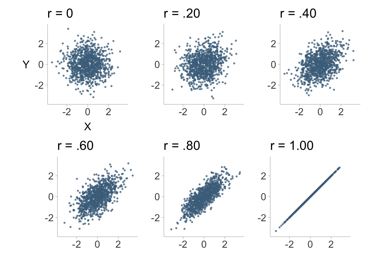
We can visualize what a correlation between two variables looks like with scatter plots. Figure 8.1 shows scatter plots with differing levels of correlation.
The standard error of the Pearson correlation coefficient is,
\[ SE_r = \sqrt{\frac{\left(1-r^2\right)^2}{n-1}} \]
Unlike Cohen’s \(d\) and other effect size measures, The correlation coefficient is bounded by -1 and positive 1, with positive 1 being a perfectly positive correlation, -1 being a perfectly negative correlation, and zero indicating no correlation between the two variables. The bounding has the consequence of making the confidence interval asymmetric around \(r\) (e.g., if the correlation is positive, the lower bound is farther away from \(r\) than the upper bound is). It is important to note that with a correlation of zero, the confidence interval is symmetric and approximately normal. To obtain the confidence intervals of \(r\), we first need to apply a Fisher’s Z transformation. A Fisher’s Z transformation is a hyperbolic arctangent transformation of a Pearson correlation coefficient and can be computed as,
\[ Z_r = \text{arctanh}(r) \]
The Fisher Z transformation ensures \(Z_r\) has a symmetric and approximately normal sampling distribution. This then allows us to calculate the confidence interval from the standard error of \(Z_r\) (\(SE_{Z_r} = \frac{1}{\sqrt{n-3}}\)),
\[ CI_{r} = Z_r \pm 1.96\times SE_{Z_r} \]
We can also back-transform the confidence interval of the Fisher’s \(Z_r\) value to obtain the confidence of the Pearson correlation,
\[ CI_{r} = \text{tanh}(CI_{Z_r}) \]
In R, the full process of obtaining the correlation and confidence intervals can be done quite easily with base R using the cor.test() function. Let’s use the palmerpenguins data set (Horst, Hill, and Gorman 2020) to look at the correlation between flipper length and body mass.
library(palmerpenguins)

# compute pearson correlation
cor.test(x = penguins$flipper_length_mm,
         y = penguins$body_mass_g,
         use = "pairwise.complete.obs", # use rows with non-missing data
         method = "pearson",
         conf.level = .95)
    Pearson's product-moment correlation

data:  penguins$flipper_length_mm and penguins$body_mass_g
t = 32.722, df = 340, p-value < 2.2e-16
alternative hypothesis: true correlation is not equal to 0
95 percent confidence interval:
 0.843041 0.894599
sample estimates:
      cor
0.8712018
The output shows that the correlation and its confidence intervals are \(r\) = 0.87, 95% CI [0.84, 0.89]. Note that you can also use the cor() function to simply get the correlation without all the extra information. We can also use the escalc() function in R to compute the correlation and CIs if all we have is the correlation and sample size (i.e., no raw data).
library(metafor)

# get pearson correlation and sample size
r <- .871
n <- 341

# calculate z-transformed correlation
stats <- escalc(measure = "ZCOR",
                ri = r,
                ni = n)

# get pearson correlation and CI
summary(stats, transf = tanh)
      yi  ci.lb  ci.ub
1 0.8710 0.8428 0.8945
8.1 Rank-Order (Spearman) Correlation
If we want to get the monotonic relationship between two variables rather than the strictly linear relationship, we can look at the correlation between ranks of \(X\) and \(Y\). A Spearman rank-order correlation is actually just the Pearson correlation on ranks such that,
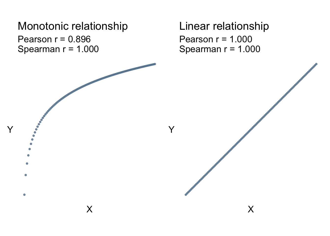
\[ r_{s} = \frac{\mathrm{Cov}(\mathrm{rank}(X),\mathrm{rank}(Y))}{S_{\mathrm{rank}(X)}S_{\mathrm{rank}(Y)}} \] Viewing Figure 8.2 we can see that non-linear monotonic relationships are captured well with Spearman’s correlation, whereas Pearson’s correlation is only describing the linear relationship between the two.
We can use base R to calculate Spearman correlations. Let’s use the palmerpenguins data set (Horst, Hill, and Gorman 2020) to look at the correlation between flipper length and body mass.
library(palmerpenguins)

# compute spearman correlation
cor(x = penguins$flipper_length_mm,
    y = penguins$body_mass_g,
    use = "pairwise.complete.obs", # use rows with non-missing data
    method = "spearman")
[1] 0.83997418.2 Concordance-Discordance (Kendall) Correlation
Similar to Spearman’s rank-order correlation, Kendall’s correlation (Kendall 1945) is a rank-based correlation that measures the ordinal association between variables. The equation for Kendall’s correlation is expressed as,
\[
r_\tau = \frac{2}{n(n-1)}\sum_{i<j} \mathrm{sign}(x_i-x_j)\cdot\mathrm{sign}(y_i-y_j)
\] Where \(i=1...n\) and \(j=1...n\) denote the observations and \(\mathrm{sign}(\cdot)\) returns the sign of whatever is in the parentheses such that a positive value returns 1, a negative value returns –1 and zero returns 0. Similar to Pearson’s and Spearman’s correlations we can compute Kendall’s correlation in base R. We will use the palmerpenguins data set again.
library(palmerpenguins)

# compute kendall correlation
cor(x = penguins$flipper_length_mm,
    y = penguins$body_mass_g,
    use = "pairwise.complete.obs", # use rows with non-missing data
    method = "kendall")
[1] 0.6604675