collaboration, confidence interval, effect size, open educational resource, open scholarship, open science
T-tests are the most commonly used statistical tests for examining differences between group means or examining a group mean against a constant. Calculating effect sizes for t-tests are fairly straightforward. Nonetheless, there are cases where statistical information for the calculation of effect sizes are missing (which happens quite often in older articles), and therefore we document methods that make use of partial information (e.g., only the mean and standard deviation, or only the t-statistic and degrees of freedom) for the calculation. There are multiple types of effect sizes used to calculate standardized mean differences (\(d\)), yet researchers very often do not identify which type of \(d\) value they are reporting (see Lakens 2013). Here we document the equations and code necessary for calculating each type of \(d\) value compiled across multiple sources (Becker 1988; Cohen 1988; Lakens 2013; Caldwell 2022; Glass, McGaw, and Smith 1981). A \(d\) value calculated from a sample will also contain sampling error, therefore we will also include equations to calculate the standard error. The standard error allows us to then calculate the confidence interval. For each variant of \(d\) in the sections below, the 95% confidence interval is calculated in the following way, that is,
\[
CI_d = d \pm 1.96\times SE
\tag{7.1}\]
Lastly, we will supply example R code so you can apply to your own data.
Here is a table for every effect size discussed in this chapter:
Uses the average within-group standard deviation to standardize the mean difference. Can be calculated directly from a independent sample t-test. Assumes homogeneity of variance between groups.
Uses the standard deviation of the control group to standardize the mean difference (often referred to as Glass’s Delta). Does not assume homogeneity of variance between treatment/intervention and control group.
Uses the standard deviation of difference scores (also known as change scores) to standardize the within person mean difference (i.e., pre/post change).
Uses the within-person standard deviation that utilizes a correction to \(d_z\) to reduce the impact of the pre/post correlation on the effect size. Assumes homogeneity of variance between conditions.
Uses the pooled variance between conditions (pre/post test). Does not use the correlation between conditions. Assumes homogeneity of variance between conditions.
Uses the pre-test standard deviation to standardize the pre/post mean difference. Does not assume homogeneity of variance between pre-test and post-test.
\(d_{PPC1}\) - Separate pre-test standard deviations
Defined as the difference between the Becker’s d between the treatment and control group. Particularly, standardizing the mean pre/post change by the pre-test of the respective group.
Standardizes the difference in mean changes between treatment and control group. Assumes homogeneity of variance between the pre-test of the control and treatment condition.
\(d_{PPC3}\) - Pooled pre-test and post-test standard deviation
Pools the standard deviation between pre-test and post-test in treatment and control condition. Assumes homogeneity of variance between pre/post-test scores and treatment and control conditions. Confidence intervals are not easy to compute.
Whatever effect size you choose to report, you can report it alongside the t-test statistics (i.e., t-value and the p value). For example,
The treatment group had a significantly higher mean than the control group (t = 2.76, p = .009, n = 35, d = 0.47, 95% CI [0.11, 0.81]).
7.2 Single Group Designs
For a single-group design, we want to compare the mean of that group to some constant, \(C\) (i.e., a target value). The standardized mean difference for a single group can be calculated by (equation 2.3.3, Cohen 1988),
\[
d_s = \frac{M-C}{S},
\tag{7.2}\]
where the standardizer (\(S\)) is the sample standard deviation. The interpretation of \(d_s\) is therefore how many standard deviations is the mean away from the target value, \(C\). A positive \(d_s\) value would indicate that the mean is larger than the target value \(C\), whereas a negative \(d_s\) value would denote the mean is less than the \(C\). The corresponding standard error for \(d_s\) can then be calculated with (see documentation for Caldwell 2022),
where \(n\) denotes the sample size. In R, we can use the d.single.t() function from the MOTE package (Buchanan et al. 2019) to calculate the single group standardized mean difference.
# Install packages if not already installed:# install.packages('MOTE')# Cohen's d for one group# For example:# Sample Mean = 30.4, SD = 22.53, N = 96# Target Value, C = 15library(MOTE)stats <-d.single.t(m =30.4,u =15,sd =22.53,n =96)SE <-sqrt(1/stats$n + stats$d^2/(2*stats$n))# print just the d value and confidence intervalsdata.frame(d =round(stats$d,3), SE =round(SE,3),ci.lb =round(stats$dlow,3), ci.ub =round(stats$dhigh,3))
      d    SE ci.lb ci.ub
1 0.684 0.113  0.46 0.904
As you can see, the output shows that the effect size is \(d_s\) = 0.68, 95% CI [0.46, 0.90].
7.3 Two Independent Groups Design
7.3.1 Standardize by Pooled Standard Deviation \((d_p)\)
For a design that consists of two independent groups (we can denote these as group \(A\) and group \(B\)), the standardized mean difference can be calculated by (equation 5.1, Glass, McGaw, and Smith 1981),
Using the pooled standard deviation as the standardizer characterizes the classic formulation of Cohen’s \(d\). This formulation requires the assumption that the variances (likewise the standard deviations) are equal between groups in the population. If this assumption is not met then it is recommended to use some of the other \(d\) value formulations later in this section. We can interpret the \(d_p\) value as the number of standard deviations the mean of group A is away from the mean of group B. A positive \(d_p\) value would indicate that the mean of group \(A\) is larger than the mean of group \(B\) and vice versa for a negative \(d_p\) value.
Cohen’s \(d_p\) is related to the t-statistic from an independent samples t-test. In fact, we can calculate the \(d_p\) value from the \(t\)-statistic with the following formula (equation 5.3, Glass, McGaw, and Smith 1981):
In R, we can use the escalc() function from the metafor package to calculate the two group standardized mean difference (using the measure = "SMD" argument).
# use metafor packagelibrary(metafor)## Standardized mean difference for two independent groups# Given means and SDs# For example:# Group A Mean = 30.4, SD = 22.53, N = 96# Group B Mean = 21.4, SD = 19.59, N = 96stats <-escalc(measure ="SMD",m1i =30.4,m2i =21.4,sd1i =22.53,sd2i =19.59,n1i =96,n2i =96,var.names =c("d", "variance") # add informative labels)# print outputsummary(stats)
       d variance    sei     zi   pval  ci.lb  ci.ub
1 0.4246   0.0213 0.1460 2.9093 0.0036 0.1386 0.7107
# Given t-test statistics# For example:# t = 2.954, nA = 96, nB = 96stats <-escalc(measure ="SMD",ti =2.954,n1i =96,n2i =96,var.names =c("d", "variance") # add informative labels)# print outputsummary(stats)
       d variance    sei     zi   pval  ci.lb  ci.ub
1 0.4247   0.0213 0.1460 2.9097 0.0036 0.1386 0.7108
The output for both examples show that the effect size is \(d_p\) = 0.42, 95% CI [0.14, 0.71].
7.3.2 Standardize by Control Group Standard Deviation (\(d_{\Delta}\))
When two groups differ substantially in their standard deviations, we can instead standardize by one of the two available group’s standard deviation, typically this is the control or reference group. In our scenario let’s suppose that group \(B\) is the control/reference group and therefore we can use the standard deviation of group \(B\) (\(S_B\)) as the standardizer, such that,
\[
d_{\Delta} = \frac{M_A-M_B}{S_B}.
\tag{7.8}\]
This formulation is commonly referred to as Glass’ \(\Delta\)(Glass 1981). The standard error for \(d_{\Delta}\) can be defined as,
Standardizing by the control group standard deviation rather than pooling (as we did in the previous section with \(d_p\)) results in less degrees of freedom (\(df=n_C-1\)) and therefore a larger standard error. In R, we can use the escalc() function from the metafor package to calculate \(d_\Delta\) (using the measure = "SMD1" argument). Since we have already loaded in the metafor package, we do not need to do it again.
# Glass' delta (standardize by control group)# given difference score means and SDs# For example:# group A Mean = 30.4, SD = 22.53, N = 96# group B Mean = 21.4, SD = 19.59, N = 96stats <-escalc(measure ="SMD1",m1i =30.4,m2i =21.4,sd2i =19.59, # Note: use sd2i for whichever group needs to be standardizedn1i =96,n2i =96,var.names =c("d", "variance") # add informative labels)# print the SDM value and confidence intervalssummary(stats)
       d variance    sei     zi   pval  ci.lb  ci.ub
1 0.4558   0.0219 0.1480 3.0788 0.0021 0.1656 0.7459
7.4 Repeated Measures Designs
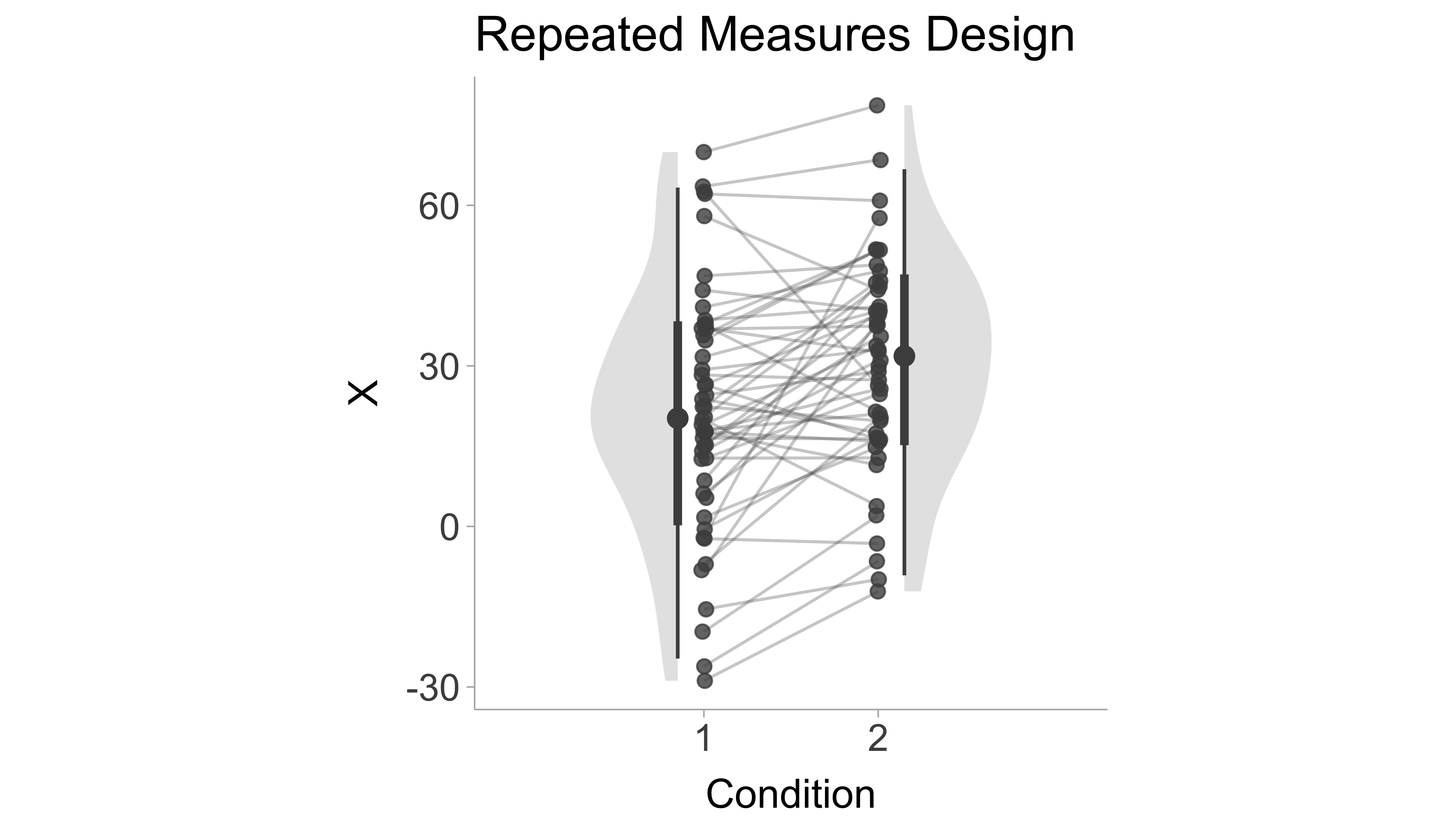
In a repeated-measures design, the same subjects (or items, etc.) are measured on two or more separate occasions, or in multiple conditions within a single session, and we want to know the mean difference between those occasions or conditions (Baayen, Davidson, and Bates 2008; Barr et al. 2013). An example of this would be in a pre/post comparison where subjects are tested before and after undergoing some treatment (see Figure 7.1 for a visualization). A standardized mean difference in a repeated-measures design can take on a few different forms that we define below.
Figure 7.1: Figure displaying simulated data of a repeated measures design, the x-axis shows the condition (e.g., pre-test and post-test) and y-axis is the scores. Lines indicate within person pre/post change.
7.4.1 Difference Score \(d\) (\(d_z\))
Instead of comparing the means of two sets of scores, a within subject design allows us to subtract the scores obtained in condition 1 from the scores in condition 2. The means and standard deviations of difference scores (\(X_{\text{diff}}=X_2-X_1\)) can be treated similarly to that of a single group design (if the target value was zero, i.e., \(C=0\)) such that (equation 2.3.5, Cohen 1988),
A positive \(d_z\) value would indicate that the scores in condition 2 are, on average, larger than scores than condition 1 and vice versa for a negative \(d_z\) value. A convenient aspect of \(d_z\) is that it has a straight-forward relationship with the paired \(t\)-statistic, \(d_z=\frac{t}{\sqrt{n}}\). This makes it very useful for power analyses. If the standard deviation of difference scores are not accessible, then it can be calculated using the standard deviation of condition 1 (\(S_1\)), the standard deviation of condition 2 (\(S_2\)), and the correlation between conditions (\(r\)) (equation 2.3.6, Cohen 1988):
\[
S_{\text{diff}}=\sqrt{S^2_1 + S^2_2 - 2 r S_1 S_2}
\tag{7.11}\]
It is important to note that when the correlation between groups is large, then the \(d_z\) value will also be larger, whereas a small correlation will return a smaller \(d_z\) value. The standard error of \(d_z\) can be calculated similarly to the single group design such that,
In R, we can use the escalc() function from the metafor package to calculate \(d_z\) (using the measure = "SMCC" argument).
# Cohen's dz for difference scores# From paired t-test# For example:# t = 10.70, N = 96stats <-escalc(measure ="SMCC",ti =10.70,ni =96,var.names =c("d", "variance") # add informative labels)# print outputsummary(stats)
       d variance    sei     zi   pval  ci.lb  ci.ub
1 1.0834   0.0165 0.1286 8.4267 <.0001 0.8314 1.3354
# given difference score means and SDs# For example:# Difference Score Mean = 21.4, SD = 19.59, N = 96stats <-escalc(measure ="SMCC",m1i =21.4,m2i =0, # per documentation, this value should be set to zerosd1i =19.59,sd2i =0, # per documentation, this value should be set to zerori =0, # per documentation, this value should be set to zeroni =96,var.names =c("d", "variance") # add informative labels)# print outputsummary(stats)
       d variance    sei     zi   pval  ci.lb  ci.ub
1 1.0837   0.0165 0.1286 8.4283 <.0001 0.8317 1.3358
The output shows that the effect size is \(d_z\) = 1.08, 95% CI [0.83, 1.34].
7.4.2 Repeated Measures \(d\) (\(d_{rm}\))
For a within-group design, we want to compare the means of scores obtained from condition 1 and condition 2. The repeated measures standardized mean difference between the two conditions can be calculated by (equation 9, Lakens 2013),
\[
d_{rm} = \frac{M_2-M_1}{S_w}.
\tag{7.13}\]
The standardizer here is the within-subject standard deviation, \(S_w\). The within-subject standard deviation can be defined as,
\[
S_{w}=\sqrt{\frac{S^2_1 + S^2_2 - 2 r S_1 S_2}{2(1-r)}}.
\tag{7.14}\]
We can also express \(S_w\) in terms of the standard deviation of difference scores (\(S_{\text{diff}}\)),
Ultimately, \(d_{rm}\) is more appropriate as an effect size estimate for use in meta-analysis whereas \(d_z\) is more appropriate for power analysis (Lakens 2013). The standard error for \(d_{rm}\) can be computed as,
In R, we can use the d.ind.t.rm function from the MOTE package to calculate the repeated measures standardized mean difference (\(d_{rm}\)).
# Cohen's d for repeated measures# given means and SDs and correlationlibrary(MOTE)# For example:# Condition 1 Mean = 30.4, SD = 22.53, N = 96# Condition 2 Mean = 21.4, SD = 19.59, N = 96# correlation between conditions: r = .40stats <-d.dep.t.rm(m1 =30.4,m2 =21.4,sd1 =22.53,sd2 =19.59,r = .40,n =96,a =0.05)SE =sqrt( (1/stats$n + stats$d^2/(2*stats$n)) *2*(1-stats$r))# print just the d value and confidence intervalsdata.frame(d =round(stats$d,3), SE =round(SE,3),ci.lb =round(stats$dlow,3), ci.ub =round(stats$dhigh,3))
      d    SE ci.lb ci.ub
1 0.425 0.117 0.215 0.633
The output shows that the effect size is \(d_{rm}\) = 0.43, 95% CI [0.22, 0.63].
7.4.3 Average Variance \(d\) (\(d_{av}\))
The problem with \(d_{z}\) and \(d_{rm}\), is that they require the correlation between conditions. In practice, correlations between conditions are frequently not reported. An alternative estimator of \(d\) in repeated measures design is to simply use the classic variation of Cohen’s \(d_p\) (i.e., pooled standard deviation). In a repeated measures design, the sample size does not change between conditions, therefore weighting the variance of condition 1 and condition 2 by their respective degrees of freedom is an unnecessary step. Instead, we can standardize by the square root of the average the variances of condition 1 and 2 (see equation 5, Algina and Keselman 2003):
This formulation is convenient especially when the correlation between conditions is not present, however without the correlation it fails to take into account the consistency of change between conditions. However, the consistency of scores is taken into account in the standard error of the \(d_{av}\) which can be expressed as (equation 9, Algina and Keselman 2003),
As we might expect, the higher the correlation (the more consistent the change in scores between conditions) the smaller the standard error. In R, we can use the escalc() function from the metafor package to calculate the average variance standardized mean difference (\(d_{av}\); using the measure = "SMCRP" argument).
# Cohen's d for repeated measures (average variance)# given means and SDs # For example:# Condition 1 Mean = 30.4, SD = 22.53, N = 96# Condition 2 Mean = 21.4, SD = 19.59, N = 96# Correlation between conditions: r = .50stats <-escalc(measure ="SMCRP",m1i =30.4,m2i =21.4, sd1i =22.53,sd2i =19.59,ri = .50,ni =96,var.names =c("d", "variance") # add informative labels)# print just the d value and confidence intervalssummary(stats)
       d variance    sei     zi   pval  ci.lb  ci.ub
1 0.4242   0.0110 0.1049 4.0442 <.0001 0.2186 0.6298
The output shows that the effect size is \(d_{av}\) = 0.42, 95% CI [0.22, 0.63].
7.4.4 Becker’s \(d\) (\(d_b\))
An even simpler variant of repeated measures \(d\) value comes from Becker (1988). Becker’s \(d\) standardizes simply by the pre-test standard deviation (we will denote the pre-test with condition 1) when the comparison is a pre/post design,
\[
d_b = \frac{M_2-M_1}{S_1}.
\tag{7.20}\]
A convenient aspect of Becker’s d is in the use of the raw score standard deviation (\(S_1\)) as the standardizer. This allows us to interpret \(d_b\) in units of standard deviations of pre-test scores, whereas for \(d_z\) and \(d_{rm}\) the interpretation of the effect size units are less clear.
We can also obtain the standard error with (equation 13, Becker 1988),
Notice that even though the formula for calculating \(d_b\) did not include the correlation coefficient, the standard error does. Using the escalc() function, we can calculate Becker’s formulation of standardized mean difference (using the measure = "SMCR" argument).
# Cohen's d for repeated measures standardized with pre-test SD (becker's d)# given means, the pre-test SDs, and the correlation# For example:# Pre-test Mean = 21.4, SD = 19.59, N = 96# Post-test Mean = 30.4, N = 96# Correlation between conditions: r = .40# NOTE: MEANS FLIPPED SO THAT M2 - M1 # (by default escalc does M1 - M2)stats <-escalc(measure ="SMCR",m1i =30.4, # post-test meanm2i =21.4, # pre-test meansd1i =22.53, # pre-test SDri = .50, ni =96,var.names =c("d", "variance") # add informative labels)# print just the d value and confidence intervalssummary(stats)
       d variance    sei     zi   pval  ci.lb  ci.ub
1 0.3963   0.0112 0.1060 3.7389 0.0002 0.1886 0.6040
The output shows that the effect size is \(d_b\) = 0.40, 95% CI [0.19, 0.60].
7.4.5 Comparing Repeated Measures \(d\) values
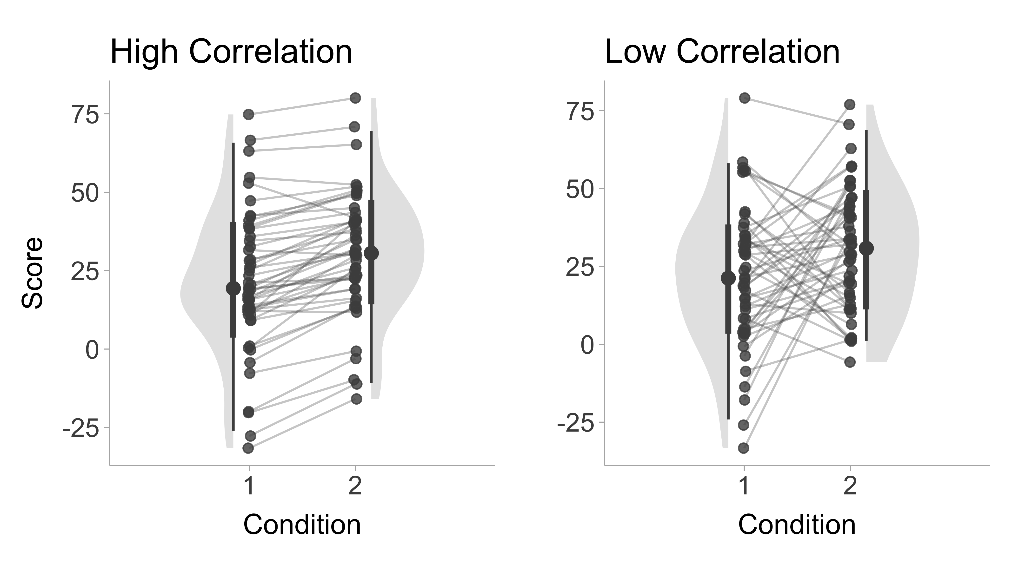
Figure 7.2 shows repeated measures designs with a high (\(r=\) .95) and low (\(r=\) .05) correlations between conditions. Let us fix the standard deviations and means for both conditions and only vary the correlation. Now we can compare the repeated measures estimators based on these two conditions shown in Figure 7.2:
High correlation:
\(d_z=1.24\)
\(d_{rm}=0.39\)
\(d_{av}=0.43\)
\(d_{b}=0.40\)
Low correlation:
\(d_z=0.31\)
\(d_{rm}=0.43\)
\(d_{av}=0.43\)
\(d_{b}=0.40\)
We notice that the correlation greatly influences \(d_z\) more than any other estimator. The \(d_{rm}\) value has very little change, whereas \(d_{av}\) and \(d_{b}\) do not take into account the correlation at all.
Figure 7.2: Figure displaying simulated data of a repeated measures design, the x-axis shows the condition (e.g., pre-test and post-test) and y-axis is the scores. Left panel shows a high pre/post correlation (\(r\) = .95) and right panel shows a low correlation condition (\(r\) = .05). Lines indicate within person pre/post change.
7.5 Pretest-Posttest-Control Group Designs
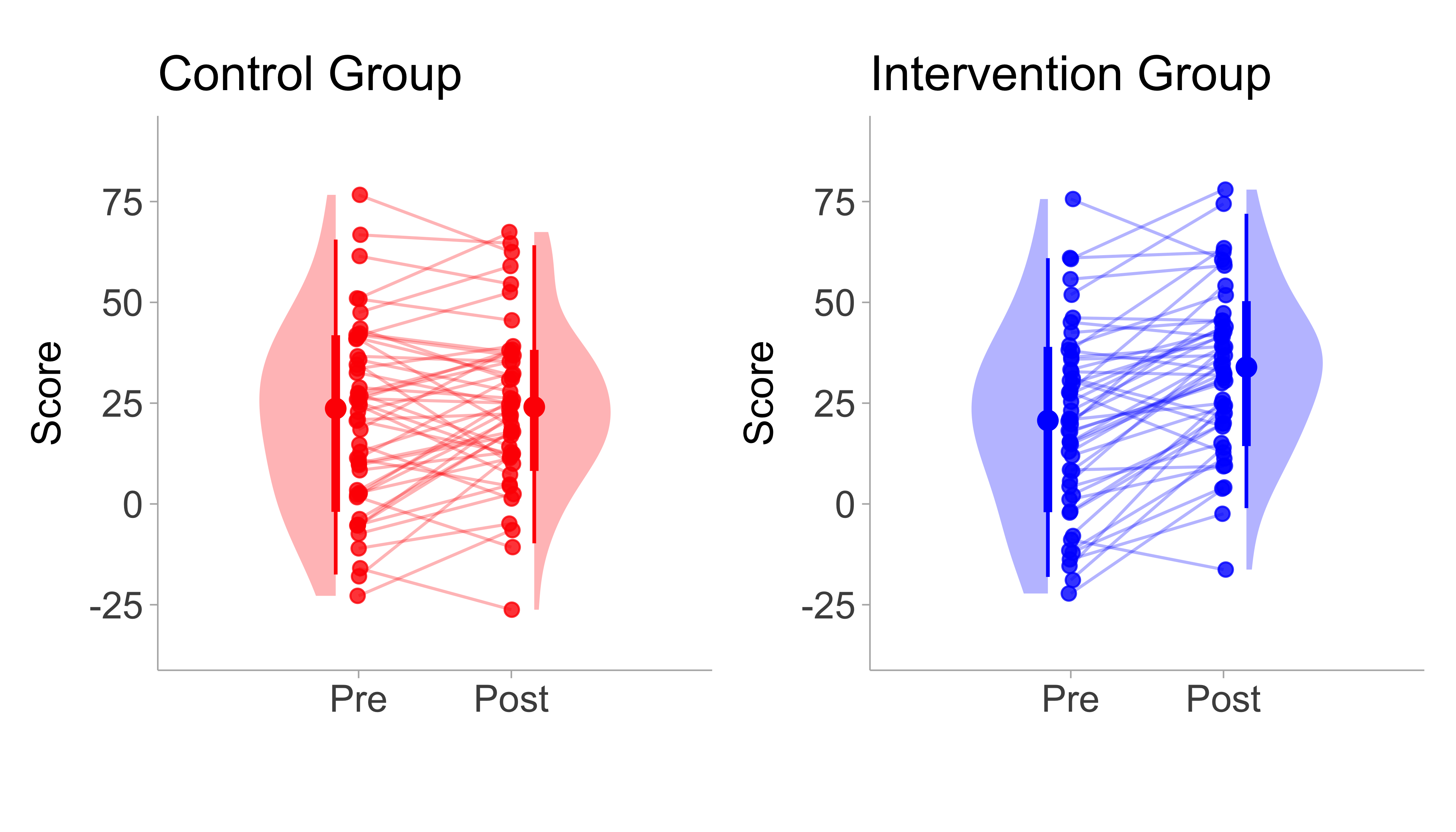
In many areas of research both between and within group factors are incorporated. For example, in research involving the examination of the effects of an intervention often a sample is randomised into two seperate groups (intervention and control) and then they are measured on the outcome of interest both before (pre-test) and after (post-test) the intervention/control period. In these types of 2x2 (group x time) study designs it is usually the difference between the standardized mean change for the intervention/treatment (\(T\)) and control (\(C\)) groups that is of interest. For a visualization of a pretest-posttest-control group design see Figure 7.3.
Morris (2008) details three effect sizes for this pretest-posttest-control (PPC).
Figure 7.3: Illustration of a pre-post control design. Left panel shows the pre-post difference in the control group and right panel shows the pre-post difference in the intervention/treatment group. Lines indicate within person pre/post change.
7.5.1 PPC1 - separate pre-test standard deviations
The separate pre-test (i.e., baseline) standard deviations are used to standardize the pre/post mean difference in the intervention group and the control group respectively (see equation 4, Morris 2008),
Note that these effect sizes are identical to the Becker’s \(d\) formulation of the SMD (see Section 7.4.4). Therefore the pretest-posttest-control group effect size is simply the difference between the intervention and control pre/post SMD (equation 15, Becker 1988),
\[
d_{PPC1} = d_T - d_C
\tag{7.24}\]
The asymptotic standard error of \(d_{PPC1}\) was first derived by Becker (1988) and can be expressed as the square root of the sum of the sampling variances (equation 16, Becker 1988),
Note that this is an approximate formula for the standard error, for an exact solution see Morris (2000). We can calculate \(d_{PPC1}\) and it’s confidence intervals using the metafor package:
# Example:# Control Group (N = 90)## Pre-test Mean = 20, SD = 6## Post-test Mean = 25, SD = 7## Pre/post correlation = .50# Intervention Group (N = 90)## Pre-test Mean = 20, SD = 5## Post-test Mean = 27, SD = 8## Pre/post correlation = .50# calculate the observed standardized mean difference# treatment group effectdT <-escalc(measure ="SMCR",m1i =27,m2i =20,sd1i =8,sd2i =5,ri = .50,ni =90)# control group effectdC <-escalc(measure ="SMCR",m1i =25,m2i =20,sd1i =7,sd2i =6,ri = .50,ni =90)# calculate d and SEdPPC1 <- dT$yi - dC$yiSE <-sqrt(dT$vi + dC$vi)# print the d value and confidence intervalsdata.frame(d =round(dPPC1,3),SE =round(SE,3),ci.lb =round(dPPC1 -1.96*SE,3),ci.ub =round(dPPC1 +1.96*SE,3))
      d    SE  ci.lb ci.ub
1 0.159 0.171 -0.176 0.494
The output shows a pre-post intervention effect of \(d_{PPC1}\) = 0.16 95% CI [-0.18, 0.49].
7.5.2 PPC2 - pooled pre-test standard deviations
The pooled pre-test (i.e., baseline) standard deviations can be used to standardized the difference in pre/post change between intervention and control groups such that (equation 8, Morris 2008),
Note the original equation shown in the paper by Morris (2008) uses the population pre/post correlation \(\rho\), however in the equation above we replace \(\rho\) with the sample size weighted average of the Pearson correlation in the treatment and control group (i.e., \(\hat{\rho} = \frac{n_T r_T + n_C r_C}{n_T + n_C}\)). Also, \(CF\) is the correction factor that can be found in the following section on small sample bias.
We can use base R to obtain \(d_{PPC2}\) and confidence intervals:
# Example:# Control Group (N = 90)## Pre-test Mean = 20, SD = 6## Post-test Mean = 25, SD = 7## Pre/post correlation = .50M_Cpre <-20M_Cpost <-25SD_Cpre <-6SD_Cpost <-7rC <- .50nC <-90# Intervention Group (N = 90)## Pre-test Mean = 20, SD = 5## Post-test Mean = 27, SD = 8## Pre/post correlation = .50M_Tpre <-20M_Tpost <-27SD_Tpre <-5SD_Tpost <-8rT <- .50nT <-90# calculate the observed standardized mean differencedPPC2 <- ((M_Tpost- M_Tpre) - (M_Cpost - M_Cpre)) /sqrt( ( (nT -1)*(SD_Tpre^2) + (nC -1)*(SD_Cpre^2) ) / (nT + nC -2) )# calculate the standard errorrho <- (nT*rT+nC*rC)/(nT + nC)CF <-gamma((nT+nC-2)/2) / ( sqrt((nT+nC-2)/2) *gamma(((nT+nC-2)-1)/2) )SE <-sqrt(2*(1-rho) * (nT+nC)/(nT*nC) * (nT+nC-2)/(nT+nC-4) * (1+ (dPPC2^2/ (2*(1- rho) * ((nT+nC)/(nT*nC))))) - dPPC2^2/CF^2)# print the d value and confidence intervalsdata.frame(d =round(dPPC2,3),SE =round(SE,3), ci.lb =round(dPPC2 -1.96*SE,3),ci.ub =round(dPPC2 +1.96*SE,3))
      d    SE ci.lb ci.ub
1 0.362 0.151 0.066 0.658
The output shows a pre-post intervention effect of \(d_{PPC2}\) = 0.36 95% CI [0.07, 0.66].
7.5.3 PPC3 - pooled pre- and post-test
The two previous effect sizes (PPC1 and PPC2) only use the pretest standard deviation and ignore the post-test standard deviation. However, if we are happy to assume that pretest and posttest variances are homogeneous1 the pooled pre-test and post-test standard deviations can be used to standardize the difference in pre/post change between intervention and control groups, such that (equation 8, Morris 2008),
The standard error for \(d_{PPC3}\) is currently unknown. An option to estimate this standard error is to use a non-parametric or parametric bootstrap by repeatedly sampling the raw data, or if the raw data is not available resample simulated data. We can do this in base R by simulating pre/post data using the mvrnorm() function from the MASS package (Venables and Ripley 2002):
# Install the package below if not done so already# install.packages(MASS)# Example:# Control Group (N = 90)## Pre-test Mean = 20, SD = 6## Post-test Mean = 25, SD = 7## Pre/post correlation = .50M_Cpre <-20M_Cpost <-25SD_Cpre <-6SD_Cpost <-7rC <- .50nC <-90# Intervention Group (N = 90)## Pre-test Mean = 20, SD = 5## Post-test Mean = 27, SD = 8## Pre/post correlation = .50M_Tpre <-20M_Tpost <-27SD_Tpre <-5SD_Tpost <-8rT <- .50nT <-90# simulate dataset.seed(1) # set seed for reproducibilityboot_dPPC3 <-c()for(i in1:1000){# simulate control group pre-post data data_C <- MASS::mvrnorm(n = nC,# input observed meansmu =c(M_Cpre,M_Cpost),# input observed covariance matrixSigma =data.frame(pre =c(SD_Cpre^2, rC*SD_Cpre*SD_Cpost), post =c(rC*SD_Cpre*SD_Cpost,SD_Cpost^2)))# simulate intervention group pre-post data data_T <- MASS::mvrnorm(n = nT,# input observed meansmu =c(M_Tpre,M_Tpost),# input observed covariance matrixSigma =data.frame(pre =c(SD_Tpre^2, rT*SD_Tpre*SD_Tpost), post =c(rT*SD_Tpre*SD_Tpost,SD_Tpost^2)))# calculate the mean difference in pre/post change (the numerator) MeanDiff <- (mean(data_T[,2]) -mean(data_T[,1])) - (mean(data_C[,2]) -mean(data_C[,1]))# calculate the pooled pre-post standard deviation (the denominator) S_Pprepost <-sqrt( ( (nT -1)*(sd(data_T[,1])^2+sd(data_T[,2])^2) + (nC -1)*(sd(data_C[,1])^2+sd(data_C[,2])^2) ) / (2*(nT + nC -2)) )# calculate the standardized mean difference for each bootstrap iteration boot_dPPC3[i] <- MeanDiff / S_Pprepost}# calculate bootstrapped standard errorSE <-sd(boot_dPPC3)# calculate the observed standardized mean differencedPPC3 <- ((M_Tpost- M_Tpre) - (M_Cpost - M_Cpre)) /sqrt( ( (nT -1)*(SD_Tpre^2+SD_Tpost^2) + (nC -1)*(SD_Cpre^2+SD_Cpost^2) ) / (2*(nT + nC -2)) )#print the d value and confidence intervalsdata.frame(d =round(dPPC3,3),SE =round(SE,3), ci.lb =round(dPPC3 -1.96*SE,3),ci.ub =round(dPPC3 +1.96*SE,3))
      d    SE ci.lb ci.ub
1 0.303 0.153 0.003 0.604
The output shows a pre-post intervention effect of \(d_{PPC3}\) = 0.30 95% CI [0.003, 0.60].
7.6 Small Sample Bias in \(d\) values
All the estimators of \(d\) listed above are biased estimates of the population \(d\) value, specifically they all over-estimate the population value in small sample sizes. To adjust for this bias, we can apply a correction factor based on the degrees of freedom. The degrees of freedom will largely depend on the estimator used. The degrees of freedom for each estimator is listed below:
Single Group design (\(d_s\)): \(df = n-1\)
Between Groups - Pooled Standard Deviation (\(d_p\)): \(df = n_A+n_B-2\)
Between Groups - Control Group Standard Deviation (\(d_\Delta\)): \(df = n_B-1\)
Pretest-Posttest-Control Separate Standard Deviation (\(d_{PPC1}\)): \(df_C=n_C−1,\; df_T=n_T−1\)
Pretest-Posttest-Control Pooled Pretest Standard Deviation (\(d_{PPC2}\)): \(df=n_T+n_C−2\)
Pretest-Posttest-Control Pooled Pretest and Posttest Standard Deviation (\(d_{PPC3}\)): \(df=2(n_T+n_C−2)\)
With the appropriate degrees of freedom, we can use the following correction factor, \(CF\), to obtain an unbiased estimate of the population standardized mean difference:
Where \(\Gamma(\cdot)\) is the gamma function. An approximation of this complex formula given by Hedges (1981) can be written as \(CF\approx 1-\frac{3}{4\cdot df -1}\). In R, this can be calculated using,
# Example (independent groups d_p):# Group 1 sample size = 20# Group 2 sample size = 18n1 <-20n2 <-18# calculate degrees of freedomdf <- n1 + n2 -2# calculate correction factorCF <-gamma(df/2) / ( sqrt(df/2) *gamma((df-1)/2) )# printCF
[1] 0.9789964
This correction factor can then be applied to any of the standardized mean difference variants mentioned above,
\[
d^* = d\times CF
\tag{7.32}\]
The corrected \(d\) value, \(d^*\), is commonly referred to as Hedges’ \(g\) or just \(g\). To avoid notation confusion we will just add an asterisk to \(d\) to denote the correction. Note that in the case of \(d_{PPC1}\), we must apply \(CF\) to both \(d_C\) and \(d_T\) such that, \(d^*_{PPC1} = d_T\times CF_T - d_C\times CF_C\). We also need to correct the standard error for \(d^*\) using the same correction factor,
\[
SE_{d^*} = SE_{d} \times CF
\tag{7.33}\]
These standard errors can then be used to calculate the confidence interval of the corrected \(d\) value,
It is very important to note that the escalc() function automatically applies the small sample correction by default, therefore any code that utilizes escalc()do not also apply the correction factor.
# Example:# Cohen's d = .50, SE = .10d = .50SE = .10# correct d value and CIs small sample biasd_corrected <- d * CFSE_corrected <- SE * CFci.lb_corrected <- d_corrected -1.96*SE_correctedci.ub_corrected <- d_corrected +1.96*SE_corrected# print just the d value and confidence intervalsdata.frame(d =round(d_corrected,3), SE = SE_corrected,ci.lb =round(ci.lb_corrected,3), ci.ub =round(ci.ub_corrected,3))
      d         SE ci.lb ci.ub
1 0.489 0.09789964 0.298 0.681
The output shows that the corrected effect size is \(d^*\) = 0.50, 95% CI [0.30, 0.68].
7.7 Ratios of Means
Another common approach, particularly within the fields of ecology and evolution, is to take the natural logarithm of the ratio between two means; the so-called Response Ratio (\(LRR\)). This is sometimes more favorable as, due to its construction using the standard deviation in some form as a denominator, the various versions of standardized mean differences are impacted by the estimate of this parameter for which studies are often less powered compared to mean magnitudes (Yang et al. 2022). For the \(LRR\) however the standard deviation only impacts its variance estimation and not the point estimate. A limitation of the \(LRR\) however is that it is limited to data that are observed on a ratio scale (i.e., have an absolute zero and instances of it are related ordinally and additively meaning both means will be positive).
Although strictly speaking the \(LRR\) is not a difference in means in an additive sense as the above standardized mean difference effect sizes are, it can in one sense be considered to reflect the difference in means on the multiplicative scale. In fact, after calculation it is often transformed to reflect the percentage difference or change between means: \(100\times \exp(LRR)-1\). However, this can introduce transformation induced bias because a non-linear transformation of a mean value is not generally equal to the mean of the transformed value. In the context of meta-analysis, when combining \(LRR\) estimates across studies a correction factor can be applied: \(100\times \exp(LRR+0.5 S^2_\text{total})-1\), where \(S^2_\text{total}\) is the variance of all \(LRR\) values.
Similarly to the various standardized mean differences, there are varied calculations for the \(LRR\) dependent upon the study design being used (see Senior, Viechtbauer, and Nakagawa 2020).
7.7.1 Response Ratio for Independent Groups (\(LRR_\text{ind}\))
When calculating the response ratio for two independent groups (group \(A\) and \(B\)). The \(LRR\) can be calculated as follows,
Using R we can easily calculate this effect size using the escalc() function in the metafor package (Viechtbauer 2010):
# LRR for two independent groups# given means and SDs# For example:# Group A Mean = 30.4, Standard deviation = 22.53, Sample size = 96# Group B Mean = 21.4, Standard deviation = 19.59, Sample size = 96# calculate lnRRind and standard errorLRRind <-escalc(measure ="ROM", m1i =30.4,m2i =21.4,sd1i =22.53,sd2i =19.59,n1i =96,n2i =96)summary(LRRind)
      yi     vi    sei     zi   pval  ci.lb  ci.ub
1 0.3511 0.0145 0.1202 2.9203 0.0035 0.1154 0.5867
The example shows a response ratio of \(LRR_\text{ind}\) = 0.35 95% CI [0.12, 0.59].
7.7.2 Response Ratio for Dependent Groups (\(LRR_\text{dep}\))
When we have dependent samples (e.g., a pre/post comparison), the \(LRR\) can be calculated as follows,
Using R we can easily calculate this effect size using the escalc() function from the metafor package as follows:
# LRR for two dependent groups# given means and SDs# For example:# Mean 1 = 30.4, Standard deviation 1 = 22.53# Mean 2 = 21.4, Standard deviation 2 = 19.59# Sample size = 96# Correlation = 0.4# calculate lnRR and standard errorLRRdep <-escalc(measure ="ROMC", m1i =30.4,m2i =21.4,sd1i =22.53,sd2i =19.59,ni =96,ri = .40)summary(LRRdep)
      yi     vi    sei     zi   pval  ci.lb  ci.ub
1 0.3511 0.0088 0.0938 3.7429 0.0002 0.1672 0.5349
The example shows a response ratio of \(LRR_\text{dep}\) = 0.35 95% CI [0.17, 0.53].
Algina, James, and H. J. Keselman. 2003. “Approximate Confidence Intervals for Effect Sizes.”Educational and Psychological Measurement 63 (4): 537–53. https://doi.org/10.1177/0013164403256358.
Baayen, R Harald, Douglas J Davidson, and Douglas M Bates. 2008. “Mixed-Effects Modeling with Crossed Random Effects for Subjects and Items.”Journal of Memory and Language 59 (4): 390–412.
Barr, Dale J, Roger Levy, Christoph Scheepers, and Harry J Tily. 2013. “Random Effects Structure for Confirmatory Hypothesis Testing: Keep It Maximal.”Journal of Memory and Language 68 (3): 255–78.
Becker, Betsy J. 1988. “Synthesizing Standardized Mean-Change Measures - UConn Library.”British Journal of Mathematical and Statistical Psychology 41 (2): 257278. https://doi.org/https://doi.org/10.1111/j.2044-8317.1988.tb00901.x.
Buchanan, Erin M., Amber Gillenwaters, John E. Scofield, and K. D. Valentine. 2019. MOTE: Measure of the Effect: Package to Assist in Effect Size Calculations and Their Confidence Intervals. http://github.com/doomlab/MOTE.
Hedges, Larry V. 1981. “Distribution Theory for Glass’s Estimator of Effect Size and Related Estimators.”Journal of Educational Statistics 6 (2): 107–28. https://doi.org/10.3102/10769986006002107.
Morris, Scott B. 2000. “Distribution of the Standardized Mean Change Effect Size for Meta-Analysis on Repeated Measures.”British Journal of Mathematical and Statistical Psychology 53 (1): 17–29.
———. 2008. “Estimating Effect Sizes From Pretest-Posttest-Control Group Designs.”Organizational Research Methods 11 (2): 364–86. https://doi.org/10.1177/1094428106291059.
Senior, Alistair M., Wolfgang Viechtbauer, and Shinichi Nakagawa. 2020. “Revisiting and Expanding the Meta-Analysis of Variation: The Log Coefficient of Variation Ratio.”Research Synthesis Methods 11 (4): 553–67. https://doi.org/10.1002/jrsm.1423.
Viechtbauer, Wolfgang. 2010. “Conducting Meta-Analyses in R with the metafor Package.”Journal of Statistical Software 36 (3): 1–48. https://doi.org/10.18637/jss.v036.i03.
Yang, Yefeng, Helmut Hillebrand, Malgorzata Lagisz, Ian Cleasby, and Shinichi Nakagawa. 2022. “Low Statistical Power and Overestimated Anthropogenic Impacts, Exacerbated by Publication Bias, Dominate Field Studies in Global Change Biology.”Global Change Biology 28 (3): 969–89. https://doi.org/10.1111/gcb.15972.
Note, this may not be the case especially where there is a mean-variance relationship and one (usually the intervention) group has a higher posttest mean score.↩︎