2 Samples, Random Variables, and Expectations
2.1 Introduction
This section is meant to provide a foundation for the rest of the book by defining concepts like populations, probability distributions, and (conditional) expectations. This section will be dense and may require some basic understanding of measure theory. This chapter does not need to be entirely understood in order to understand the rest of the book, however some of the notation used in later chapters will be introduced here. I make sure to frequently reiterate what the meaning of the notation throughout the book, so not much should be lost if this chapter is skipped.
2.2 The Sample Space and Target Population
Let \((\Psi,\mathcal{F}_\Psi)\) be a measurable space. The set \(\Psi\) is a sample space and, in our case, the population of interest. Each \(\psi \in \Psi\) is an experimental object of study such as an individual person or animal. Throughout the text \(\psi\) will most often be referred to as an “individual”, but take note that this encompasses any experimental object of interest. The \(\sigma\)-field \(\mathcal{F}_\Psi\) is a collection of measurable subsets of \(\Psi\) that is closed under complement as well as countable unions and intersections.
Let \((\Omega,\mathcal{F}_\Omega)\) also be a measurable space. The set \(\Omega\) is the outcome space where each \(\omega\in\Omega\) is a possible outcome. The \(\sigma\)–field \(\mathcal{F}_\Omega\) is the collection of measurable subsets.

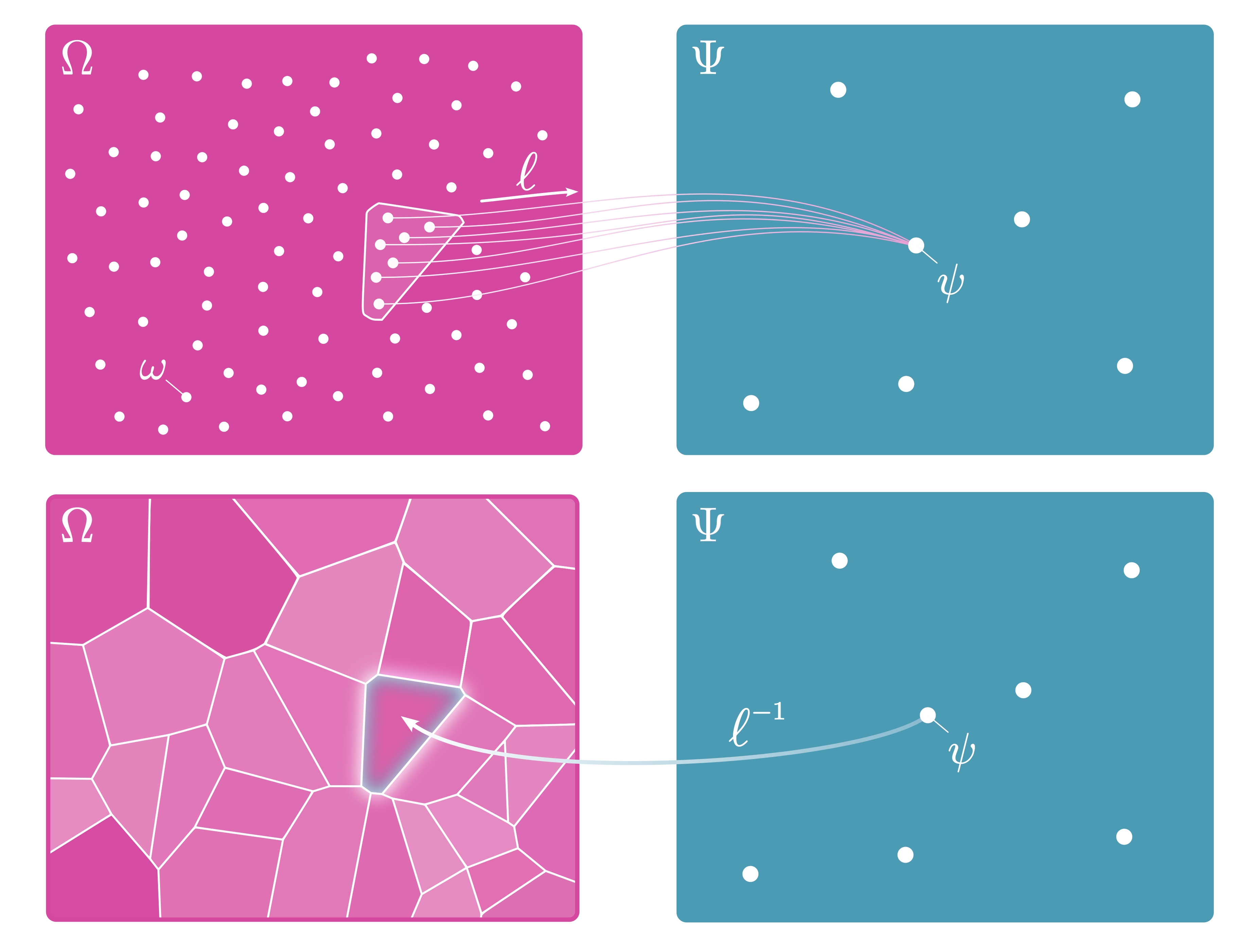
Let \(\ell\) be an assignment-to-individual function that maps the sample space \(\Omega\) to the population of interest \(\Psi\) (Zimmerman 1975; Kroc and Zumbo 2020),
\[ \ell: (\Omega,\mathcal{F}_\Omega) \rightarrow (\Psi,\mathcal{F}_\Psi). \]
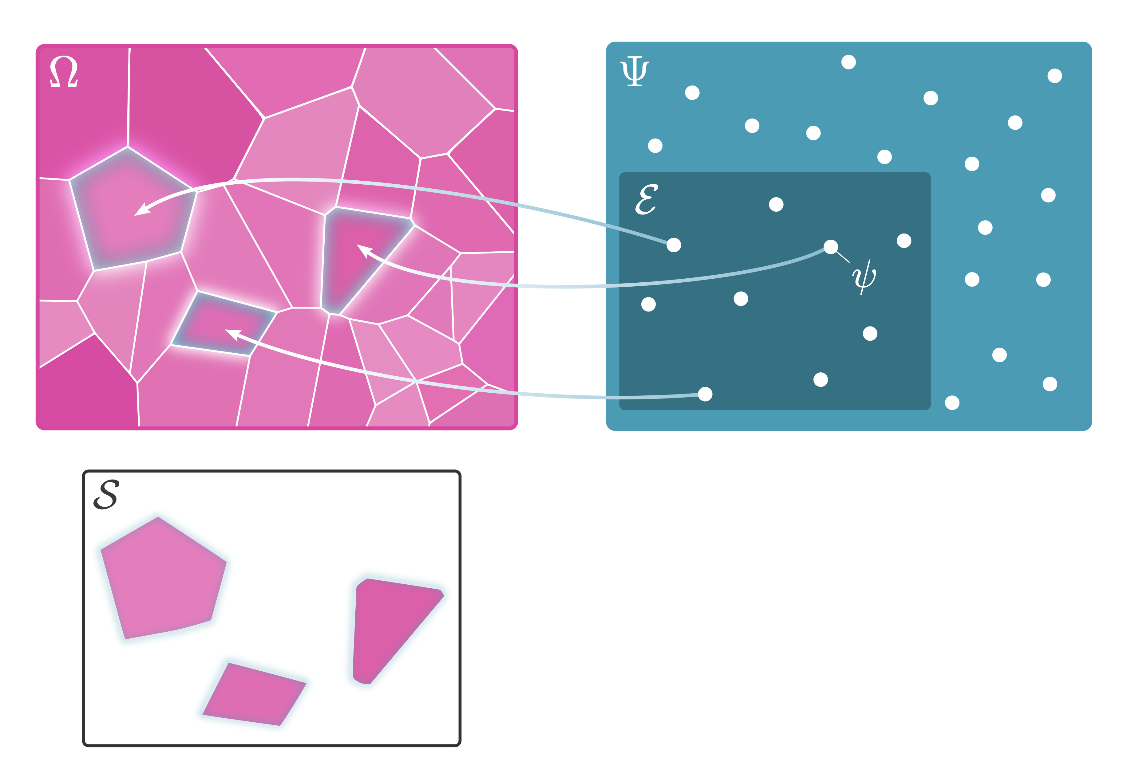
The function \(\ell\) is \(\mathcal{F}\)-measurable such that \(\ell^{-1}(\psi) \in \mathcal{F}_{\Omega}\). The preimage of an individual \(\psi\in\Psi\) under the assignment-to-individual function is also known as a fiber and encapsulates all possible outcomes for given individual (see Figure 2.2). We can union the fibers of \(\ell\) to recover the total sample space such that \(\Omega = \bigcup_{\psi\in\Psi}\ell^{-1}(\psi)\).
2.3 Random Variables and Measurement Error
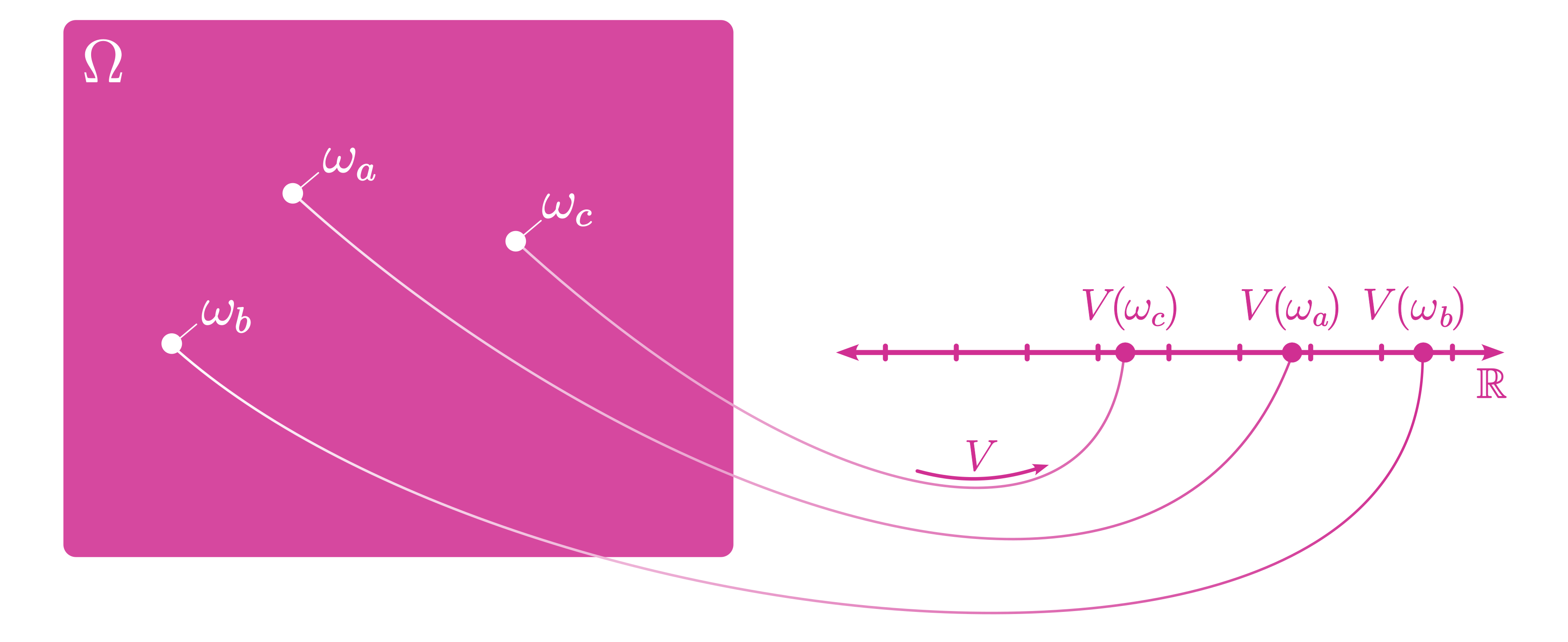
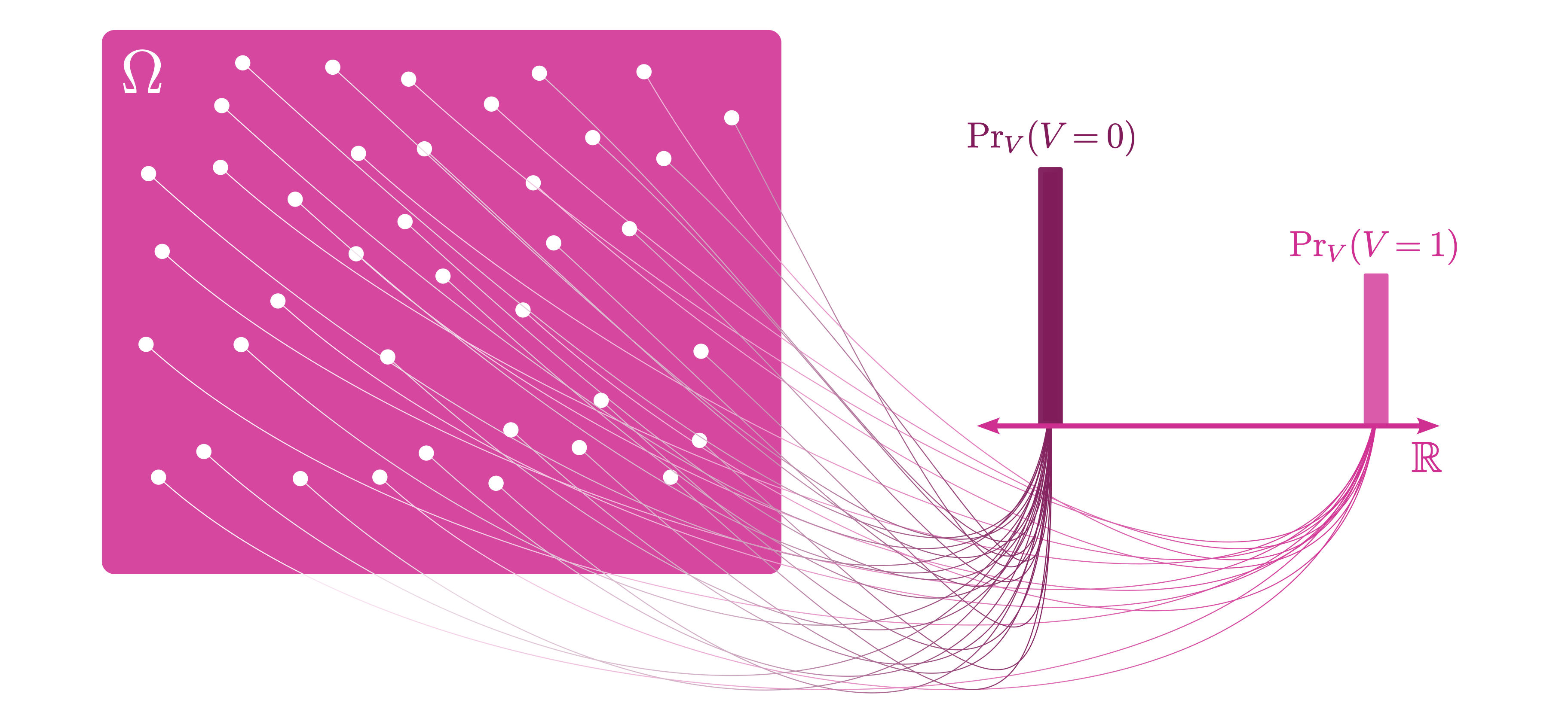
The sample units in the sample space are arbitrarily valued, but we can convert them to real number values by defining a random variable, that is, a function that takes each \(\omega\in\Omega\) and assigns it a real-valued quantity. A real-valued random variable \(V\) is a measurable function that maps the probability space \((\Omega,\mathcal{F}_\Omega,{\Pr}_V)\) equipped with a probability measure \({\Pr}_V\) to the set of real numbers equipped with the Borel \(\sigma\)–field (i.e., the smallest \(\sigma\)–field containing all open sets; see Figure 2.3),
\[ V: (\Omega,\mathcal{F}_\Omega,{\Pr}_V) \rightarrow (\mathbb{R},\mathcal{B}_\mathbb{R}). \]
Where the probability of the sample space is \({\Pr}_V(\Omega)=1\). The random variable is \((\mathcal{F}_\Omega,\mathcal{B}_\mathbb{R})\)–measurable such that \(V^{-1}(B)\in\mathcal{F}_\Omega\) for all \(B\in\mathcal{B}_\mathbb{R}\).
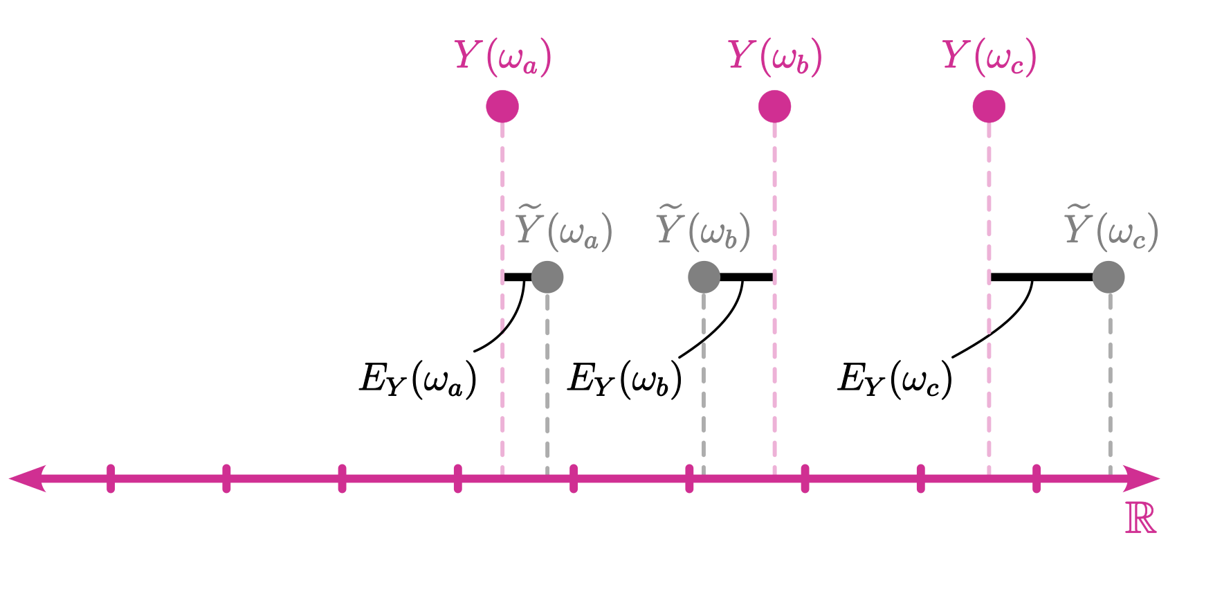
We can now define the relevant random variables that will be used over the course of the book. Let \(Y\) be a random variable of scientific interest (i.e., the measurand) denoting our dependent variable (i.e., the outcome variable). For real-world studies, we often are unable to observe the true value of \(Y\) directly and instead we must rely on drawing inferences about the true value from a error-prone proxy \(\widetilde{Y}\) that is obtained from a measurement procedure. Clearly if the measurement procedure does not produce any error then \(\widetilde{Y}(\omega) = Y(\omega)\) for each \(\omega\in\Omega\). If the measurement procedure contains measurement error then there will be differences between the true value \(Y\) and outcomes of the measurement \(\widetilde{Y}\). We can specify an algebraic structure relating the proxy \(\widetilde{Y}\) to the true value \(Y\),
\[ \widetilde{Y} = Y + E_Y \tag{2.1}\]
Where \(E_Y\) is the measurement error term defined as the difference between the error-prone proxy and the true value \(E_Y = \widetilde{Y} - Y\) (see Figure 2.4).For this book, the random variable \(Y\) will be continuous such that for any outcome \(\omega\in\Omega\) the random variables take on real values, \(Y(\omega) \in \mathbb{R}\).
The set of all possible measurement outcomes for an individual \(\psi\in\Psi\) can be written as \(\widetilde{Y}(\ell^{-1}(\psi))\in\mathcal{F}_\Omega\). Over these possible measurement outcomes, we will assume that the dependent variable of interest \(Y\) stays constant across all outcomes for an individual such that \(Y(\omega_\mathsf{a})=Y(\omega_\mathsf{b})\) if \(\omega_\mathsf{a},\omega_\mathsf{b} \in \ell^{-1}(\psi)\) whereas the measured proxy variable may not, \(\widetilde{Y}(\omega_\mathsf{a})\neq \widetilde{Y}(\omega_\mathsf{b})\). This is a property of true scores most often associated with Classical Test Theory (Kroc and Zumbo 2020), which may not be optimal for many applications such as longitudinal studies where true scores are expected to change over time within a person.
We also want to define two independent variables \(X\) and \(G\) of interest and structure them in an algebraically similar manner to Equation 2.1,
\[ \widetilde{X} = X + E_X \tag{2.2}\]
\[ \widetilde{G} = G + E_G \tag{2.3}\]
Where \(X\) is a continuous random variable similar to \(Y\) and thus also takes on real values whereas \(G\) is a Bernoulli random variable and takes the value of either 0 or 1, \(G(\omega)\in\{0,1\}\). Measurement errors for Bernoulli random variables are usually referred to as misclassifications (see chapter on group misclassification).
2.4 Probability Distributions and Density Functions
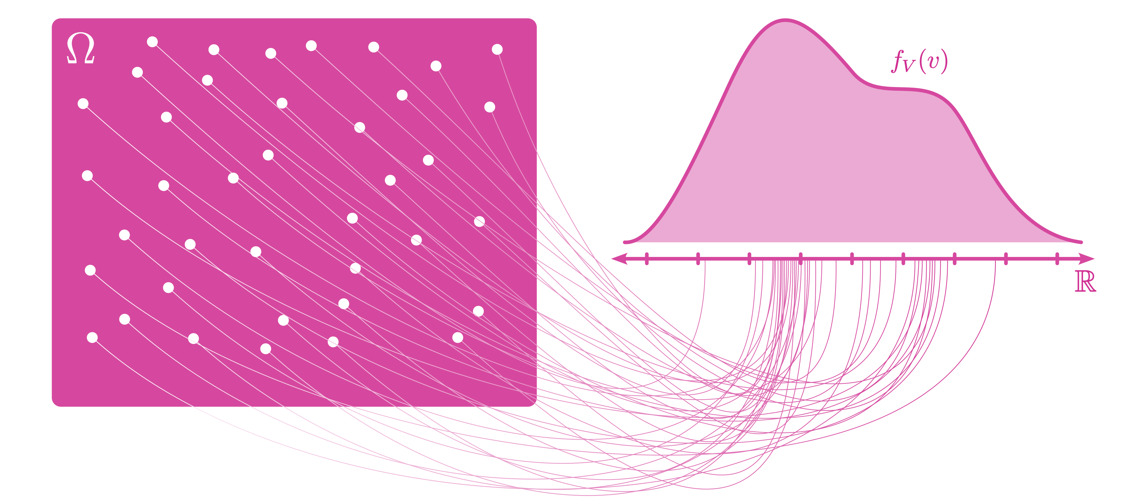
The probability distribution of a random variable allows us to assign probabilities to most subsets of the real line. The probability distribution of a continuous random variable \(V\) can often (except in mostly pathological cases) be described by a probability density function \(f_V\) (see Figure 2.5). The probability density function \(f_V\) is a nonnegative function that satisfies,
\[ {\Pr}_V(V\in\mathbb{R}) = \int_\mathbb{R} f_V(v)\, dv = 1. \tag{2.4}\]
In other words, the probability of \(V\) taking on a value anywhere on the real line is 1 (i.e., no uncertainty in that statement). To obtain the probability that \(V\) exists in some Borel subset \(B \subset \mathbb{R}\) of the real line (e.g., an interval), we can integrate the probability density function \(f_V\) over \(B\),
\[ {\Pr}_V(V\in B) = \int_{B\subset \mathbb{R}} f_V(v)\, dv. \tag{2.5}\]
Assume random variables \(X\) and \(Y\) (along with the associated proxies and errors) are continuous and their probability distributions can both be described by their respective probability density functions \(f_X\) and \(f_Y\). However the distribution of a Bernoulli random variable \(G\) is be described by a probability mass function (Figure 2.6),
\[ f_G(g) = p_G^g (1-p_G)^{1-g} \tag{2.6}\]
Where the parameter \(p_G\) denotes the probability that \(G=1\). Therefore the probability distribution of 0 or 1 can explicitly written out as,
\[ {\Pr}_G(G = 1) = p_G \;\;\; \text{and} \;\;\; {\Pr}_G(G = 0) = 1-p_G. \]
2.5 Study Samples
For a researcher to make inferences about parameters in the population of interest, they must draw a sample of individuals from the population. Ideally, sampling is done at random in order to produce unbiased estimates of the population parameters. In practice however, this is usually not possible. In cognitive and behavioral sciences, many studies are conducted on convenience samples that are sampled from a narrow subset of the population of interest. A non-random sample may not (on average) share the same composition of characteristics as the population of interest and thus may produce biased estimates of population parameters. Here we define a study sample \(\mathcal{S}\) as a subset of the sample space consisting of the possible outcomes of individuals drawn from the set of eligible individuals (i.e., individuals the researcher has access to). Let \(\mathcal{E}\subseteq \Psi\) be the study population, that is, full set of eligible individuals. The study sample \(\mathcal{S}\) is the set of possible values from a random draw of \(n\) eligible individuals,
\[ \mathcal{S} := \bigcup^{n}_{i=1} \ell^{-1}(\psi_i)\, ,\;\;\;\; \psi_i = \psi_1...\psi_n \in_\text{R} \mathcal{E}\subseteq{\Psi} \] where \(\in_\text{R}\) denotes a random draw from a set. The eligibility of an individual (i.e., the members that constitute the study population \(\mathcal{E}\)) will be defined more precisely in the chapters on selection effects.
2.6 Conditional Expectations and Variance of Random Variables
The expectation of a random variable is a probability weighted average (i.e., the mean) over all possible sample units in the sample space. This can be defined with the Lebesgue integral of \(V\) with respect to the probability measure \({\Pr_V}\),
\[ \mathbb{E}\left[V\right] = \int_\Omega V \, d\,{\Pr}_V. \tag{2.7}\]
The expected value can be interpreted as the population mean which will be denoted as \(\mu_{V}:=\mathbb{E}(V)\). The population variance \(\sigma^2_{V}\) is the expectation of the squared deviation from it’s mean of the random variable \(V\) and can be expressed as,
\[ \sigma^2_{V} := \mathbb{E}\left[V^2\right] - \mathbb{E}\left[V\vphantom{^2}\right]^2. \]
The standard deviation of a random variable is the square root of the variance, \(\sigma_V\). The conditional expectation on the other hand is the mean over a subset of the sample space. For example, the expectation of \(Y\) given the subset of the sample space \(\Omega\) where \(G=1\) can be expressed as,
\[ \mu_{Y|G=1} :=\mathbb{E}\left[ Y \mid G^{-1}(1)\right] = \int_{G^{-1}(1)} Y \, d\,{\Pr}_{Y|G}, \]
where \({\Pr}_{Y|G}\) is the conditional probability measure.Then the conditional variance of \(Y\) given \(G=1\) is,
\[ \sigma^2_{Y|G=1} := \mathbb{E}\left[Y^2\mid G^{-1}(1) \right] - \mathbb{E}\left[Y\mid G^{-1}(1) \right]^2. \] The study population mean of \(V\) is the the expectation over the possible outcomes of all individuals in the study population \(\mathcal{E}\) can be defined as,
\[ \mu_{V|\mathcal{E}} := \mathbb{E}\left[V\mid \ell^{-1}(\mathcal{E})\right] \]
and the study population variance of \(V\) is,
\[ \sigma^2_{Y|\mathcal{E}} := \mathbb{E}\left[Y^2\mid \ell^{-1}(\mathcal{E}) \right] - \mathbb{E}\left[Y\mid \ell^{-1}(\mathcal{E})\right]^2. \]
It is worth noting that if the study population encompasses all individuals in the population of interest (i.e., all individuals in the population of interest are eligible to be sampled), then \(\mathcal{E}=\Psi\). This would indicate that the study population mean is equal to the target population mean \(\mu_{V} = \mu_{V|\mathcal{E}}\).
The expectation conditioned on a study sample \(\mathbb{E}[\,\cdot\,|\mathcal{S}]\) can be construed as a random variable that has its own probability distribution due to the random action in the study sample (i.e., the study sample is created from \(n\) random draws from the eligible pool of individuals). The expectation over a sample is interpreted as a sample estimate of the mean,
\[ m_{V} := \mathbb{E}\left[V \mid \mathcal{S}\right] = \frac{1}{n}\sum_{1...n} V_i . \]
Where \(V_i\) denotes the value of the random variable for each individual drawn from the population. Where the sample variance is,
\[ s_{V} := \mathbb{E}\left[V^2\,|\,\mathcal{S}\right] - \mathbb{E}\left[V\,|\,\mathcal{S}\vphantom{S^2}\right]^2. \]
Sample estimates of parameters will always be denoted as English letters. The covariance between two random variables \(X\) and \(Y\) is the product of the differences from the mean for each respective variable and can be expressed as,
\[ \sigma_{XY} := \mathbb{E}[XY] - \mathbb{E}[X]\mathbb{E}[Y] \]
The sample covariance can similarly defined using conditional expectations,
\[ s_{XY} := \mathbb{E}[XY\,|\,\mathcal{S}] - \mathbb{E}[X\,|\,\mathcal{S}]\,\mathbb{E}[Y\,|\,\mathcal{S}] \]