7  Artificial Dichotomization

7.1 Introduction

Researchers occasionally split naturally continuous variables into two discrete groups to increase interpretability or conduct specific analyses (e.g., t-tests). However, artificially dichotomizing variables introduces measurement error and thus attenuating effect size estimates Maxwell and Delaney (1993). The obvious solution to this problem is to simply not dichotomize variables, however if only summary data is available to us, then we may not have this luxury.

7.2 Artificial Dichotomization Induced Measurement Error

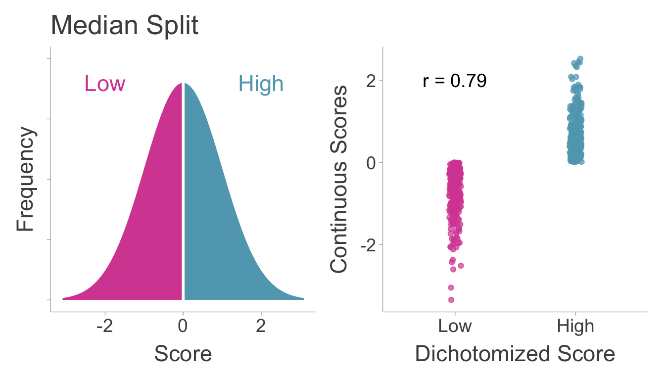
Variables that are dichotomized contain measurement error. This can be demonstrated by the simple fact that dichotomized scores are not perfectly correlated with their underlying continuous scores. To demonstrate this, we can draw a sample of scores and then split the data into high and low scorers and then calculate the correlation coefficient between the two (see Figure 7.1). We see that the dichotomized score does not perfectly correlate with it’s underlying continuous score.

Figure 7.1: Visualizing the loss of precision when artificially dichotomizing. Left panel shows a normally distributed variable split (at the median/mean) into a high scoring group and a low scoring group.

Even with a perfectly reliable measure, dichotomization will introduce measurement error. Dichotomization occurs when data is split into two groups (low and high groups will be denoted as \(\mathsf{low}\) and \(\mathsf{high}\), respectively) depending on whether they are above or below some cut-point \(c\). We can define artificially dichotomized scores as,

\[ \widetilde{X}= \begin{cases} \mathsf{high},& \text{if } \widetilde{X}\geq c\\ \mathsf{low},& \text{if } \widetilde{X}<c \end{cases} \]

7.3 Correcting Correlations for Artificial Dichotomization

7.3.1 Defining the Target Quantity

We want to obtain the population correlation between continuous scores of the independent (\(X\)) and dependent variable (\(Y\)), \(\rho_{XY}\).

There are two cases of dichotomization that may occur in a given study: the univariate case where only one variable (either \(X\) or \(Y\)) is dichotomized and the bivariate case where both variables are dichotomized. In either case, dichotomization will have a biasing effect on the study correlation coefficient. The study correlation on dichotomized data (using the bivariate case, \(r_{\widetilde{X}\widetilde{Y}}\)) can be modeled as a function of the population correlation on continuous scores (\(\rho_{XY}\); i.e., the target), an artifact attenuation factor \(\alpha\), and sampling error, \(\varepsilon_r\),

\[ r_{\widetilde{X}\widetilde{Y}} = \alpha\rho_{XY}+\varepsilon_r. \]

7.3.2 Artifact Correction for Correlations

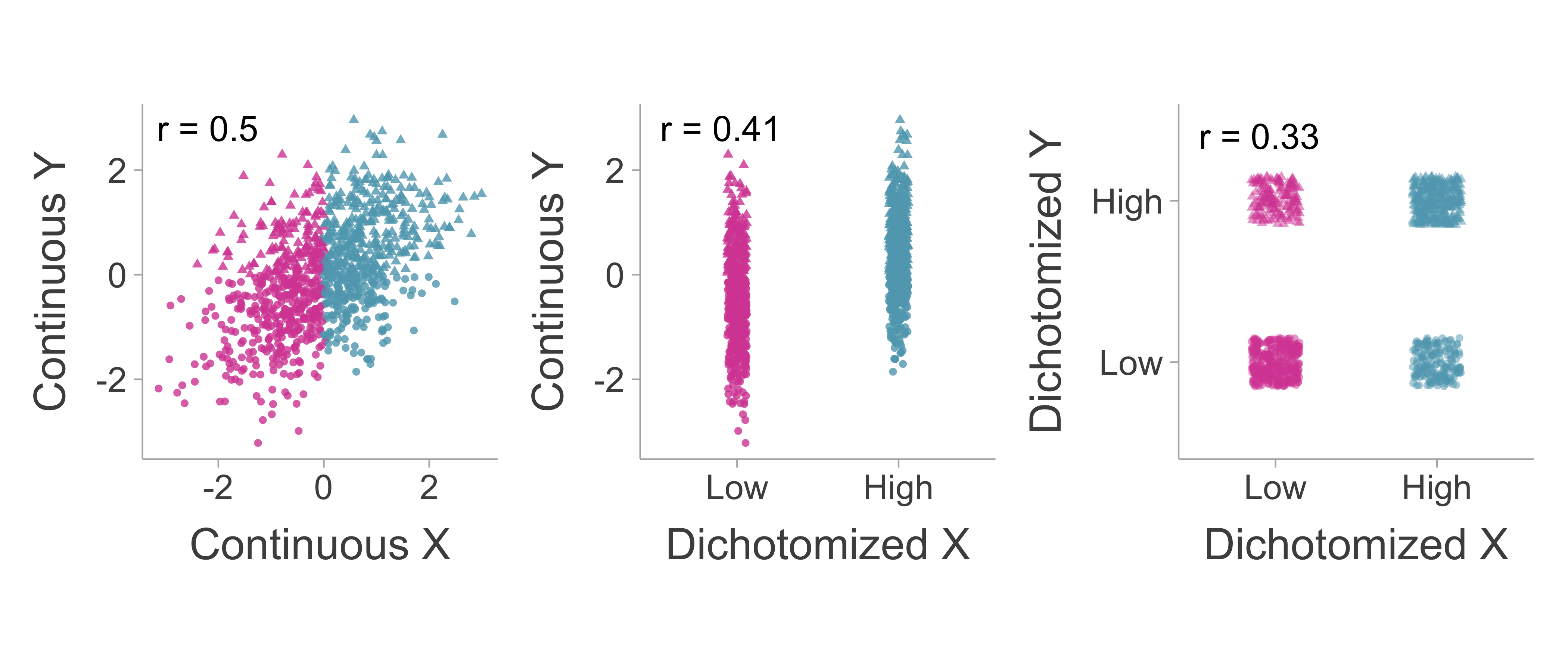
Correlations can suffer from dichotomization in one variable (univariate case) or both variables (bivariate case). This section will discuss the procedure for obtaining an unbiased estimate of the correlation coefficient for both cases. For a comparative visualization of a correlation with no dichotomization, univariate dichotomization, and bivariate dichotomization, see Figure 7.2.

Figure 7.2: Scatter plots showing the correlation under dichotomization. The first panel (left to right) shows the correlation with no dichotomization (color and shapes of points denote where the split in the dichotomized cases will occur). The middle panel shows the univariate case where only the independent variable is dichotomized. The last panel shows the bivariate case where both independent and dependent variables are dichotomized.

The Univariate Case

In the simplest case of dichotomization, only one variable is dichotomized and the other is left continuous. As mentioned in previous chapters, a Pearson correlation between a dichotomous variable and a continuous variable is a point-biserial correlation. However, if the variable is naturally continuous, we can estimate the correlation of the underlying continuous scores by computing a biserial correlation. If all we have access to is the dichotomized data, then we need to assume the shape of the underlying distribution, the biserial correlation assumes bivariate normality.

In the population, the study correlation \(\rho_{\widetilde{X} Y}\) is biased by some artifact biasing factor, \(\alpha\),

\[ \rho_{\widetilde{X} Y} = \alpha\rho_{XY}. \]

To estimate the attenuation factor \(\alpha\), we must first figure out where the split of the data occured. To do this, we must first calculate the proportion of the sample in the assigned to the low or high scoring group [^1: It will not matter whether you calculate the proportion of the sample in the high scoring group or the low scoring group for \(p_X\). Once you decide on one, do not change it.] :

\[ p_\widetilde{X} = \frac{ n_{\mathsf{high}} }{n_{\mathsf{high}} + n_{\mathsf{low}}}, \]

Where \(n\) indicates the sample size within the \(\mathsf{high}\) and \(\mathsf{low}\), scoring groups.

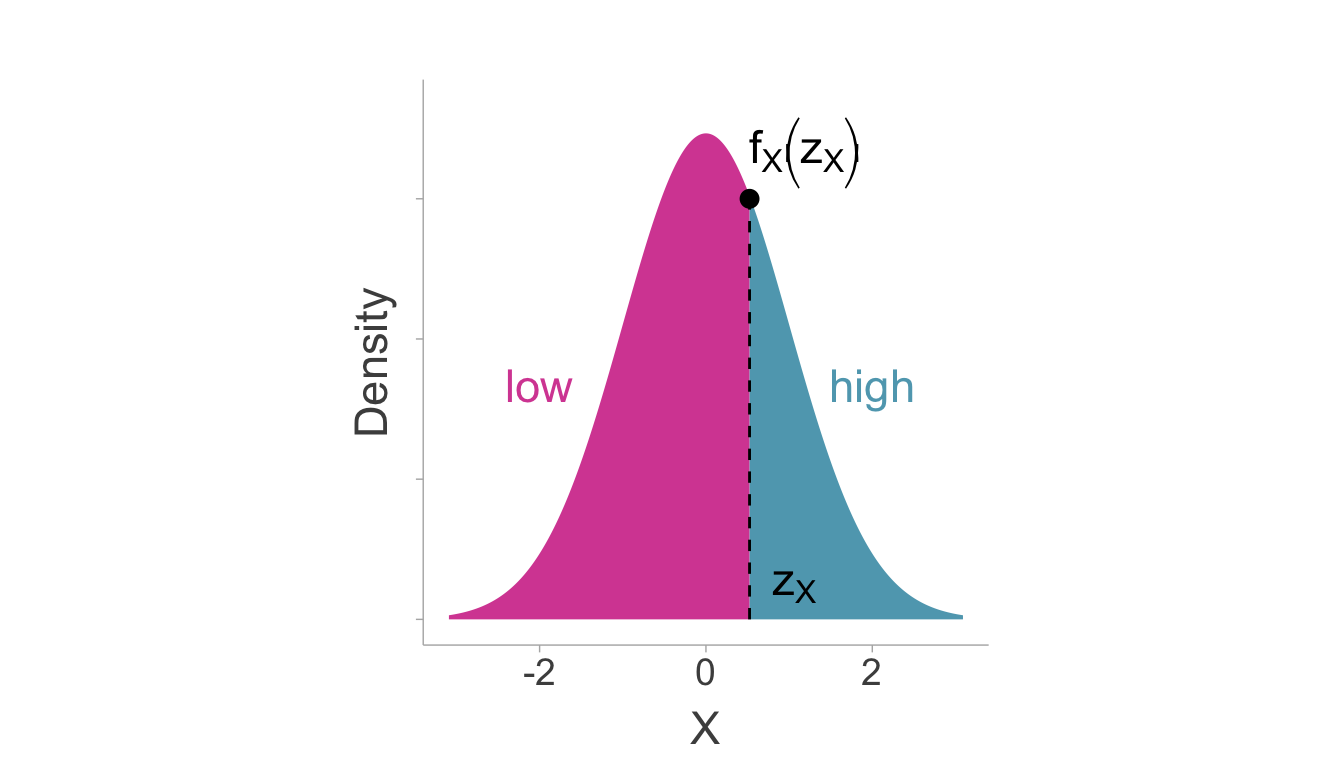
We can use the quantile function (\(\phi^{-1}[\cdot]\), i.e., the inverse of the cumulative density of the standard normal distribution) to find where the split would have occured on a standard normal distribution (i.e., z-score), \(\mathrm{z}_X=\phi^{-1}[p_X]\). Using the location of the split on the standard normal, we can compute the artifact attenuation factor [an adaptation of equation 2, Hunter and Schmidt (1990)],

\[ \hat{a} =\frac{f_X\left(\mathrm{z}_X\right)}{\sqrt{p_\widetilde{X}(1-p_\widetilde{X})}}. \tag{7.1}\]

Where \(f_X(\cdot)\) is the normal ordinate function (i.e., probability density function of a standard normal distribution). Figure 7.3 visually demonstrates how each of these relate to a standard normal distribution.

Figure 7.3: This figure shows a normal distribution of scores split into a high scoring and low scoring group. The cut-point of the standard normal distribution is computed with the quantile function, \(\phi^{-1}[p_X]\). The ordinate of the normal distribution at that cut-point is calculated with the normal ordinate function, \(\varphi\left(\phi^{-1}[p_X]\right)\).

We can correct the study correlation using the estimated artifact factor, \(\hat{a}\), therefore the full correction equation is,

\[ r_{XY} = \frac{r_{\widetilde{X}Y}}{\alpha} = \frac{r_{\widetilde{X}Y}}{\left[\frac{f_X\left(\mathrm{z}_X\right)}{\sqrt{p_\widetilde{X}(1-p_\widetilde{X})}}\right]}. \tag{7.2}\]

In the case of a median split, where the cut-point would be placed at zero of a standard normal (splitting the distribution in equal halves), the attenuation factor would simplify to \(\hat{\alpha} =\frac{\varphi(0)}{\sqrt{.5(.5)}}\) \(=\frac{2}{\sqrt{2\pi}}\approx .80\).

What to do when correlation is unavailable

It is common that studies do not report the correlation between dichotomized and continuous scores, \(r_{\widetilde{X}Y}\) (i.e., the point-biserial correlation), instead they may report the means and standard deviations of the high and low group instead. To obtain the point-biserial correlation, \(r_{\widetilde{X} Y}\), we need the the mean of the high scoring group (\(m_{Y|\mathsf{high}}\)), mean of the low scoring groups (\(m_{Y|\mathsf{low}}\)), the standard deviation of \(Y\) across all individuals (\(s_Y\); not to be confused with the pooled/average standard deviation within each group), and the sample sizes within each group (\(n_{\mathsf{high}}\) and \(n_\mathsf{low}\)) to calculate \(r_{\widetilde{X}Y}\),

\[ r_{\widetilde{X} Y} =\frac{m_{Y|\mathsf{high}}-m_{Y|\mathsf{low}}}{s_Y} \sqrt{p_\widetilde{X}(1-p_\widetilde{X})}. \]

Hunter and Schmidt (1990) suggested that one should correct the standard error by dividing the uncorrected standard error by the artifact attenuation factor (see equation 6, Hunter and Schmidt 1990). However simulations have found that this computation does not work as well as Soper’s exact method (Soper 1914; Jacobs and Viechtbauer 2017). Therefore the standard error of the corrected (biserial) correlation can be estimated with the following formula (equation 12, Jacobs and Viechtbauer 2017),

\[ \mathrm{var}(r_{XY}) = \frac{1}{n-1} \left(r_{\widetilde{X}Y}^4+r_{\widetilde{X}Y}^2\left(\frac{p_\widetilde{X}(1-p_\widetilde{X})\mathrm{z}_\widetilde{X}^2}{\varphi\left(s_X\right)^2} + \frac{2p_\widetilde{X} - 1}{f_X\left(\mathrm{z}_\widetilde{X}\right)} -\frac{5}{2}\right)+\frac{p_\widetilde{X}(1-p_\widetilde{X})}{f_X\left(\mathrm{z}_\widetilde{X}\right)^2}\right). \]

Soper (1914) also developed an approximation of the above formula,

\[ se(r_{XY}) \approx \sqrt{\frac{1}{n-1}} \left(\frac{\sqrt{p_\widetilde{X}(1-p_\widetilde{X})}}{\varphi\left(\mathrm{z}_\widetilde{X}\right)}-r_{\widetilde{X}Y}^2\right). \]

Applied Example in R

Let’s say we want to assess the relationship between a sales person’s score on a job knowledge test and their job performance estimated as the number of sales made per week. However the researchers of the study chose to dichotomize sales people into high sales performers and low sales performers by splitting the sample into two equally sized groups. They then reported the means and standard deviations of job knowledge test scores of both groups:

1. Low sales performers: Mean = 22 (SD = 4, n = 50)
2. High sales performers: Mean = 24 (SD = 4, n = 50)

To calculate the corrected correlation we can use escalc() function from the metafor package (metafor?). Using the argument measure='RBIS' will return the biserial correlation coefficient which is equivalent to the corrected correlation.

library(metafor)

escalc(measure = 'RBIS',
       m1i = 24, # High performer mean 
       m2i = 22, # Low performer mean
       sd1i = 4, # High performer SD
       sd2i = 4, # Low performer SD
       n1i = 50, # High performer sample size
       n2i = 50, # Low performer sample size
       var.names = c('rXY','var'),
       digits = 3)

    rXY   var 
1 0.307 0.014 

Therefore the estimated correlation on continuous scores is \(r_{XY}=.31\).

If the study reported a Pearson correlation (point-biserial) between the dichotomized variable and the continuous variable of \(r_{\widetilde{X} Y}=.245\), then

library(psychmeta)

correct_r_dich(r = .245, # study point-biserial correlation
               px = .50, # proportion of sample in low or high group
               n = 100) # total sample size

  r_corrected var_e_corrected    n_adj
1    0.307062      0.01401901 59.51455

The corrected correlation for continuous scores is equal to the calculation using the means and standard deviations.

The Bivariate Case

In some cases, both independent and dependent variables are dichotomized. A Pearson correlation calculated on these two dichotomized (binary) variables would be equal to the phi coefficient (or also known as Matthew’s correlation coefficient) and we can denote it with our notation for dichotomized variables, \(\rho_{\widetilde{X}\widetilde{Y}}\). Dichotomized data can be structured in a contingency table (see Table 7.1).

Table 7.1: Contingency table.

	\(\widetilde{X}=\mathrm{low}\)	\(\widetilde{X}=\mathrm{high}\)
\(\widetilde{Y}=\mathrm{low}\)	\(n_{LL}\)	\(n_{HL}\)
\(\widetilde{Y}=\mathrm{high}\)	\(n_{LH}\)	\(n_{HH}\)

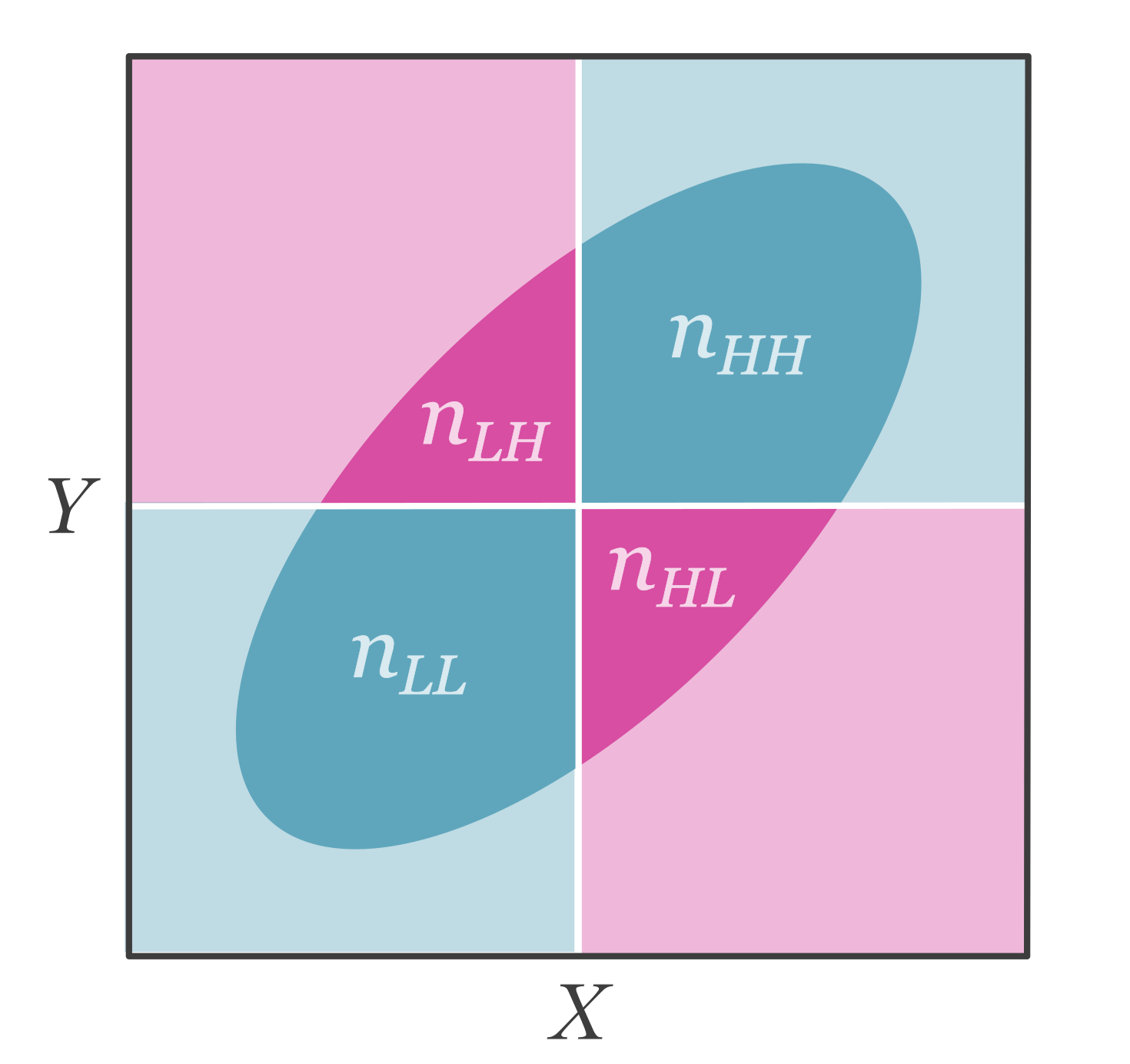
Figure 7.4 illustrates how this contingency table relates to an underlying continuous bivariate normal distribution.

Figure 7.4: The ellipse indicates the bivariate normal distribution of \(X\) and \(Y\) with a strong positive correlation. If \(X\) and \(Y\) are positively correlated then we should more individuals populating the high-high and low-low cells rather than the high-low and low-high cells which can be seen by the area of the ellipse located in each quadrant.

The corrected correlation coefficient for two dichotomized variables is commonly referred to as the tetrachoric correlation coefficient. The tetrachoric correlation estimates the correlation on continuous scores assuming a bivariate normal distribution.

One of the difficulties of computing a dichotomization corrected (tetrachoric) correlation (\(r_{XY}\)) is that the relationship between binary variables is reported very differently, we will describe how to obtain a dichtomization corrected correlation in four different cases:

1. The full contingency table is provided, including the sample sizes for each cell.
2. The odds ratio is reported as well as the marginal proportions (proportions in low and high groups for each variable).
3. The Phi coefficient is reported.

Case 1: Full contingency table is reported

If the full contingency table is reported, then the tetrachoric correlation can be calculated directly. Due to the complexity of the calculation, we will use R.

The escalc() function in the metafor package (Viechtbauer 2010) can take on values from a contingency table and compute a tetrachoric correlation using the measure='RTET' argument. The function uses the method described by Kirk (1973).

# Example Contingency Table
#    XL   XH
# YL 43   23
# YH 27   38  

library(metafor)

escalc(measure = 'RTET',
       ai = 43,
       bi = 23,
       ci = 27,
       di = 38,
       var.names = c('rXY','se.2'))

     rXY   se.2 
1 0.3637 0.0155 

The results show a dichotomization corrected correlation of \(r_{XY} = .36\) and an estimated sampling variance of \(se_c^2=.016\).

Case 2: odds ratio is reported

If the odds ratio is all that is available, then we can use the tetrachoric correlation approximation described by Bonett and Price (2005). Using the estimated odds ratio (\(OR=(n_{HH}n_{LL})/(n_{HL}n_{LH})\)) and the marginal proportions (\(p_X\) and \(p_Y\); for this case, both proportions should be with respect to the high scoring group) we can approximate the dichotomization corrected (tetrachoric) correlation (see equation 4, Bonett and Price 2005),

\[ r_{XY} \approx \cos\left( \frac{\pi}{1+OR^\gamma}\right) \] Where \(\Omega\) is

\[ \gamma = 1 - \frac{\left|p_\widetilde{X} -p_\widetilde{Y}\right|}{5} - \left[\frac{1}{2}-\min(p_\widetilde{X},p_\widetilde{Y})\right]^2. \]

Note that \(\min(p_X,p_Y)\) is the smallest marginal proportion. The standard error of the estimated correlation can be computed with the following formula [see equation 9, Bonett and Price (2005); note this equation is slightly changed in order to account for the fact that we only have access to the marginal sample sizes and proportions]

\[ se(r_{XY}) = \left(\frac{\pi\times \gamma\times OR^\gamma\times\sin\left(\frac{\pi}{1+OR^\gamma}\right)}{\left(1+OR^\gamma\right)^2}\right)^2\times\frac{4}{n} \]

Where \(n\) is the total sample size. Using base R, we can convert the odds ratio to a tetrachoric correlation.

pX <- .4 # proportion of individuals in high group in XD
pY <- .5 # proportion of individuals in high group in YD
n <- 150 # total sample size
OR <- 1.43 # odds ratio
gamma_factor <- 1 - abs(pX-pY) / 5 - (1/2 - min(c(pX,pY)))^2

# calculate corrected correlation
rXY <- cos(pi/(1+OR^gamma_factor))

# calculate standard error
var_r <- (pi*gamma_factor*OR^gamma_factor*sin(pi/(1+OR^gamma_factor)) /
  ((1+OR^gamma_factor)^2))^2 * 4/n

cbind(rXY, var_r)

           rXY      var_r
[1,] 0.2665276 0.01354199

Case 3: Correlation between dichotomized variables

A Pearson correlation coefficient calculated between two binary variables is most commonly referred to as a Phi coefficient or Matthew’s correlation coefficient. However, the Phi coefficient underestimates the correlation on the underlying continuous scores (assuming bivariate normality). Therefore we can approximate the correlation on continuous scores by using a similar correction to the univariate case. We can define an artifact attenuation factor that is similar to Equation 7.1, but with the added attenuation of \(\widetilde{Y}\),

\[ \alpha =\left[\frac{f_X\left(\mathrm{z}_X\right)}{\sqrt{p_\widetilde{X}(1-p_\widetilde{X})}}\right]\times\left[\frac{f_Y\left(\mathrm{z}_Y\right)}{\sqrt{p_\widetilde{Y}(1-p_\widetilde{Y})}}\right]. \]

Therefore we can correct \(r_{\widetilde{X}\widetilde{Y}}\) for dichotomization in both variables by dividing by the attenuation factor,

\[ r_{XY} = \frac{r_{\widetilde{X}\widetilde{Y}}}{\alpha}=\frac{r_{\widetilde{X}\widetilde{Y}}}{\left[\frac{f_X\left(\mathrm{z}_X\right)}{\sqrt{p_\widetilde{X}(1-p_\widetilde{X})}}\right]\times\left[\frac{f_Y\left(\mathrm{z}_Y\right)}{\sqrt{p_\widetilde{Y}(1-p_\widetilde{Y})}}\right]} \]

This correction is only an approximation, however it performs fairly well when the correlation is below .8 (Hunter and Schmidt 1990). The standard error of the corrected correlation can be calculated similarly (adaptation of equation 9, Hunter and Schmidt 1990),

\[ \mathrm{var}(r_{XY})=\frac{se(r_{\widetilde{X}\widetilde{Y}})}{\left[\frac{f_X\left(\mathrm{z}_X\right)}{\sqrt{p_\widetilde{X}(1-p_\widetilde{X})}}\right]^2\times\left[\frac{f_Y\left(\mathrm{z}_Y\right)}{\sqrt{p_\widetilde{Y}(1-p_\widetilde{Y})}}\right]^2} \]

Using the correct_r_dich() function in the psychmeta package (dahlke2019?), we can correct the observed study correlation for dichotomization.

library(psychmeta)

correct_r_dich(r = .20,  # observed study correlation
               px = .50, # proportion of sample in high group of XD
               py = .50, # proportion of sample in high group of YD
               n = 100)  # sample size

  r_corrected var_e_corrected    n_adj
1   0.3141593      0.02296926 36.36678

The output shows the corrected correlation to be \(r_{XY}=.31\) and it’s estimated sampling variance \(\mathrm{var}(r_{XY})=.023\).

7.4 Correcting Standardized Mean Differences (SMDs)

7.4.1 Defining our Target SMD

The target quantity is the standardized mean difference between groups of a naturally continuous variable. Our target can thus be defined as the population standardized mean difference between groups \(A\) and \(B\) on continuous scores of the dependent variable, \(\delta_{gY}\). For a given study the dichotomized standardized mean difference (\(d_{gY_D}\)) can be defined as,

\[ d_{G\widetilde{Y}} = \alpha\delta_{GY} + \varepsilon_d \] where \(\alpha\) is the artifact attenuation factor and \(\varepsilon_d\) is the sampling error.

7.4.2 Artifact Correction for SMD

The simplest way to correct for dichotomization in a standardized mean difference is to first convert the observed \(d_{G\widetilde{Y}}\) value of the dichotomized dependent variable to a correlation coefficient. When converting to a correlation coefficient, it’s important to note the binary nature of both variables. Now when we convert the SMD to a correlation it will be the phi coefficient rather than the point-biserial correlation that we would be estimating if the dependent variable was continuous. To calculate the phi coefficient from a \(d_{GY}\) value we can use the proportion of group membership in group 0 or 1 (\(p_G\); it does not matter which one is chosen, as long as it is consistent),

\[ r_{G\widetilde{Y}} = \frac{d_{G\widetilde{Y}}}{\sqrt{d_{G\widetilde{Y}}^2+\frac{1}{p_G(1-p_G)}}} \]

We can then correct the correlation similar to how we did in Section 7.3.2,

\[ r_{GY} = \frac{r_{G\widetilde{Y}}}{\left[\frac{f_Y\left(\mathrm{z}_Y\right)}{\sqrt{p_\widetilde{Y}(1-p_\widetilde{Y})}}\right]}. \]

Then we can convert the corrected correlation back into a standardized mean difference,

\[ d_{GY} = \frac{r_{GY}}{\sqrt{p_G\left(1-p_G\right)\left(1-r_{GY}^2\right)}}. \]

Where \(d_{GY}\) is our corrected SMD (i.e., the estimated SMD on continuous variables). The observed sampling variance must also be corrected using the same three step procedure. For simplicity, we will consolidate this into one formula,

\[ \mathrm{var}(d_{GY}) = \frac{\mathrm{var}(d_{G\widetilde{Y}}) \times \frac{r_{GY}}{r_{G\widetilde{Y}}} } {\left(1+d_{G\widetilde{Y}}^2p_G[1-p_G]\right)^3(1-r_{GY}^2)^3}. \]

Obtaining Standardized Mean Difference from Odds Ratio

In most cases, difference in dichotomized outcomes between two groups is unlikely to be reported as a standardized mean difference, instead it will be more commonly reported as an odds ratio (\(OR\)). The odds ratio is asymmetric about 1 (i.e., the null), but we can make it symmetric by log transforming it (\(\log(OR)\)). The standard error of the log odds ratio can be defined as,

\[ \mathrm{var}(\log(OR)) = \frac{1}{n_{1H}} + \frac{1}{n_{1L}} + \frac{1}{n_{0H}} + \frac{1}{n_{0L}} \]

The equation above requires the full contingency table to compute. From there we can use the cox-logit method to convert the odds ratio to a standardized mean difference (Cox 1989; Haddock, Rindskopf, and Shadish 1998). Them method is quite simple as it just divides the log odds ratio by 1.65,

\[ d_{GY} = \frac{\log(OR)}{1.65} \tag{7.3}\]

and the corresponding sampling variance of the \(d\) value is,

\[ \mathrm{var}(d_{GY}) = \frac{\mathrm{var}(\log(OR))}{1.65}. \]

Applied Example in R

Let’s consider a hypothetical scenario where we want to examine the relationship between caffeine consumption and the occurrence of heart palpitations in a population. Our target quantity in this case is the standardized mean difference of coffee consumption between people with and without heart palpitations. The variable of interest, caffeine consumption, is continuous (measured in milligrams per day). However, the researcher decides to dichotomize this variable into two groups: “High Caffeine Consumers” and “Low Caffeine Consumers.”

Suppose we have a sample of 500 individuals, and we dichotomize their caffeine consumption into “High Caffeine Consumers” (more than 250mg per day) and “Low Caffeine Consumers” (less than or equal to 250mg per day). We also observe the occurrence of heart palpitations in these individuals.

	Heart Palpitations: Yes	Heart Palpitations: No
High Consumers	60	140
Low Consumers	20	280

We can calculate the dichotomization corrected standardized mean difference by calculating the log odds ratio with escalc() function and then applying Equation 7.3 to estimate \(d_{gY}\).

# calculate log-odds ratio
OR <- escalc(measure = 'OR',
             ai = 60,
             bi = 140,
             ci = 20,
             di = 280,
             var.names = c('logOR','var'))  

# convert to standardized mean difference
dGY <- OR$logOR / 1.65
var_d <- OR$var / 1.65

# print results
cbind(dGY,var_d)

          dGY      var_d
[1,] 1.085915 0.04689755

We can see that the standardized mean difference is estimated to be \(d_{GY}=1.09\) and the corrected standard error is \(\mathrm{var}(d_{GY})=.047\)

Bonett, Douglas G., and Robert M. Price. 2005. “Inferential Methods for the Tetrachoric Correlation Coefficient.” Journal of Educational and Behavioral Statistics 30 (2): 213–25. https://www.jstor.org/stable/3701350.

Cox, D. R. 1989. Analysis of Binary Data. 2nd ed. New York: Routledge. https://doi.org/10.1201/9781315137391.

Haddock, C. Keith, David Rindskopf, and William R. Shadish. 1998. “Using Odds Ratios as Effect Sizes for Meta-Analysis of Dichotomous Data: A Primer on Methods and Issues.” Psychological Methods 3 (3): 339–53. https://doi.org/10.1037/1082-989X.3.3.339.

Hunter, John, and Frank Schmidt. 1990. “Dichotomization of Continuous Variables: The Implications for Meta-Analysis.” Journal of Applied Psychology 75 (June): 334–49. https://doi.org/10.1037/0021-9010.75.3.334.

Jacobs, Perke, and Wolfgang Viechtbauer. 2017. “Estimation of the Biserial Correlation and Its Sampling Variance for Use in Meta-Analysis.” Research Synthesis Methods 8 (2): 161–80. https://doi.org/10.1002/jrsm.1218.

Kirk, David B. 1973. “On the Numerical Approximation of the Bivariate Normal (Tetrachoric) Correlation Coefficient.” Psychometrika 38 (2): 259–68. https://doi.org/10.1007/BF02291118.

Maxwell, Scott, and Harold Delaney. 1993. “Bivariate Median Splits and Spurious Statistical Significance.” Psychological Bulletin 113 (January): 181–90. https://doi.org/10.1037/0033-2909.113.1.181.

Soper, H. E. 1914. “On the Probable Error of the Bi-Serial Expression for the Correlation Coefficient.” Biometrika 10 (2/3): 384–90. https://doi.org/10.2307/2331789.

Viechtbauer, Wolfgang. 2010. “Conducting meta-analyses in R with the metafor package.” Journal of Statistical Software 36 (3): 1–48. https://doi.org/10.18637/jss.v036.i03.